refinepeaks
Syntax
Description
[
refines peaks based on a signal with amplitudes yRPeaks,xRPeaks] = refinepeaks(y,xPeaksIdx)y, and indices of the
initial peak estimates xPeaksIdx, returning the refined peak values
yRPeaks and location estimates xRPeaks. This
syntax uses quadratic least squares processing to refine the peaks based on
xRPeaks and two surrounding points for every selected peak.
[___] = refinepeaks(___,
specifies additional options, such as the peak refinement method and method specifications,
using name-value arguments. Use this syntax with any of the input or output arguments in
preceding syntaxes.Name=Value)
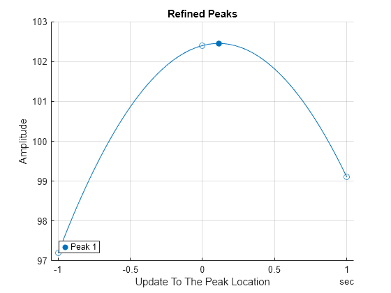
refinepeaks(___) with no output arguments draws a
figure that compares the refined peak amplitudes and locations to the initial peak estimates
and their surrounding samples. The figure also plots the fitting curves used to refine the
peaks. The refinepeaks function plots the three-point sets with
unfilled circles and plots the refined peaks with filled circles.
Examples
Refine a known peak from a signal specified as a vector or as a MATLAB® timetable.
Create a five-element vector. Set the fourth sample so that it is a local maximum. Plot the function and observe that the fourth sample is a signal peak with an amplitude of 102.4.
Intensity = [100;98.7;97.2;102.4;99.1];
plot(Intensity)
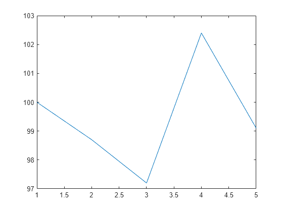
Refine the known peak and compute its refined value and location. The refined peak is located slightly after the original peak on the fourth sample of the signal.
[YRpeak,XRpeak] = refinepeaks(Intensity,4)
YRpeak =
102.4531
XRpeak =
4.1118
Create a timetable from a signal, using a sample rate of 1 Hz.
TT = timetable(Intensity,SampleRate=1)
TT=5×1 timetable
    Time     Intensity
    _____    _________

    0 sec        100
    1 sec       98.7
    2 sec       97.2
    3 sec      102.4
    4 sec       99.1
Refine the peak and plot the result. Observe that the refined peak occurs 0.11 seconds after the initial estimate, and the refined peak value of 102.45 shows as a filled circle. The original peak is at 0 seconds for reference, while the surrounding points are at -1 second and 1 second from the reference.
refinepeaks(TT,4)
Generate a Rayleigh distribution with a scale parameter b set to .
P = @(x,b) (x/b^2).*exp(-0.5*(x/b).^2);
x = 0:2.5:20;
b = pi;
p = P(x,b);
plot(x,p)
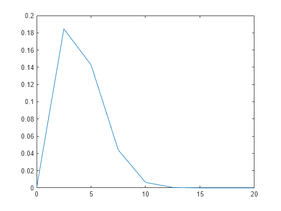
Calculate the theoretical and estimated peak amplitude and location. The peak is located about half of a sample from the expected peak scaled location, .
yPeakTheo = P(b,b);
xPeakTheo = b;
yPeakEst = max(p);
xPeakIdx = find(p==max(p));
xPeakEst = x(xPeakIdx);
disp(table(["Estimated";"Theoretical"], ...
    [yPeakEst;yPeakTheo],[xPeakEst;xPeakTheo], ...
    VariableNames=["Peak" "Amplitude" "Location"]))
        Peak         Amplitude    Location
    _____________    _________    ________

    "Estimated"       0.18456         2.5
    "Theoretical"     0.19306      3.1416
Refine the peak estimation using the quadratic least squares (QLS) method with default specifications.
[yRPeakDef,xRPeakDef] = refinepeaks(p,xPeakIdx,x);
Refine the peak estimation using the QLS method by specifying an exponential kernel with an exponent value of three.
[yPeakRef,xPeakRef] = refinepeaks(p,xPeakIdx,x, ...
    Method="QLS",QLSKernel="exp",KernelPower=3);
Compare the peak refinement results. The refined peak amplitude and location with both QLS-method variants yield a better approximation of the theoretical values than do the initial estimates. The exponential kernel yields the best approximation of the peak theoretical values for the specified Rayleigh distribution.
disp(table(["Initial Estimation";"Refined (QLS default)"; ...
    "Refined (QLS customized)";"Theoretical"], ...
    [yPeakEst;yRPeakDef;yPeakRef;yPeakTheo], ...
    [xPeakEst;xRPeakDef;xPeakRef;xPeakTheo], ...
    VariableNames=["Peak" "Amplitude" "Location"]))
               Peak               Amplitude    Location
    __________________________    _________    ________

    "Initial Estimation"           0.18456         2.5
    "Refined (QLS default)"        0.19581      3.2884
    "Refined (QLS customized)"     0.19315      3.2398
    "Theoretical"                  0.19306      3.1416
Obtain a refined peak location estimate for the main two peaks in a signal using the nonlinear least squares method with a sinc function kernel.
Generate Signal
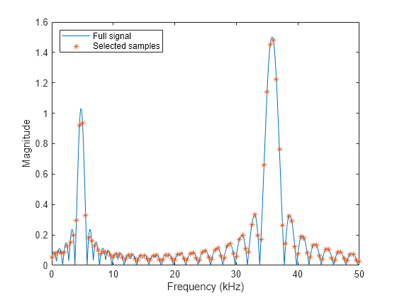
Radar pulse compression of a linear FM waveform produces a sinc-shaped spectrum, where the frequency locations of the peaks are proportional to the distance between the radar and the detected object. You can first estimate the peak locations and amplitudes with findpeaks and then enhance your estimates with refinepeaks. This example finds the peak amplitudes and locations of a synthetic noiseless pulse compression signal and uses refinepeaks to improve the estimates.
Generate a signal composed of two sinc-shaped waveforms with peaks of 1 and 1.5 at 4.76 kHz and 35.8 kHz, respectively. Set the frequency spacing to 2.5 Hz.
aTg = [1 1.5];
fTg = 1e3*[4.76 35.8];
freqkHzFull = (0:0.0025:50)';
waveFull = abs(sinc([1 0.5].*(freqkHzFull-fTg/1e3)))*aTg';
Downsample the signal by a factor of 200 so the frequency spacing between samples is 0.5 kHz. This example refines the amplitude and location estimates of the downsampled signal peaks and compares the improved estimates to the values in the original signals.
freq = downsample(freqkHzFull,200);
wave = downsample(waveFull,200);

plot(freqkHzFull,waveFull,freq,wave,"*")
legend(["Full signal" "Selected samples"],Location="northwest")
xlabel("Frequency (kHz)")
ylabel("Magnitude")
Refine Peaks Using Nonlinear Least Squares
Use findpeaks to make initial estimates of the amplitudes, locations, and half-height widths of the two highest peaks of the signal.
[PV,PL,PW] = findpeaks(wave,NPeaks=2, ...
    SortStr="descend",WidthReference="halfheight");
table(PV,freq(PL), RowNames="Peak estimate "+(1:numel(PV)), ...
    VariableNames=["Amplitude" "Frequency (kHz)"])
ans=2×2 table
                       Amplitude    Frequency (kHz)
                       _________    _______________

    Peak estimate 1     1.4824            36
    Peak estimate 2     0.9374             5
Use refinepeaks to enhance the peak estimation using the nonlinear least squares (NLS) method. Specify the frequency points of the signal and the peak widths. The peak values are significantly closer to the expected values of 1.5 and 1, while the frequency locations approximate well to 35.8 kHz and 4.76 kHz, respectively.
LW = max(PW,2);
[Ypk,Xpk] = refinepeaks(wave,PL,freq,Method="NLS",LobeWidth=LW);
table(Ypk,Xpk, RowNames="Refined peak "+(1:numel(Ypk)), ...
    VariableNames=["Amplitude" "Frequency (kHz)"])
ans=2×2 table
                      Amplitude    Frequency (kHz)
                      _________    _______________

    Refined peak 1     1.5063            35.8
    Refined peak 2     1.0163          4.7628
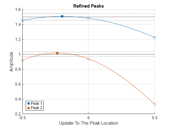
Plot the amplitudes of the refined peaks on the y-axis and the updated peak locations compared with the initial peak estimates on the x-axis. The two initially estimated peaks and their two surrounding samples are each separated by 0.5 kHz. The refined peaks, indicated by filled circles, show the actual peak locations compared to the initially estimated peak locations as well as the corrected amplitudes.
refinepeaks(wave,PL,freq,Method="NLS",LobeWidth=LW)
yline(aTg) % Theoretical peak amplitudes
errorBounds = aTg.*(1+0.03*[-1;1]);
yline(errorBounds(:),":") % ±3% error bounds
legend("Peak "+[1 2])
Identify and refine peaks from hourly temperature data across rows, columns, and pages.
Plot Data
Load a MAT file containing a set of temperature readings in degrees Celsius taken every hour at Boston Logan International Airport for the entire month of January 2011.
load bostemp
tempArray = (tempC(1:24*28))';
timeArray = 1 + (0:numel(tempArray)-1)/24;
Reshape the data from the first 28 days into a three-dimensional array with 24 rows (hours of the day), 7 columns (weekdays), and 4 pages (weeks).
temps3D = reshape(tempArray,[24 7 4]);
times3D = reshape(timeArray,[24 7 4]);
Plot the temperatures across weeks.
temps2D = reshape(temps3D,[24*7 4]);
times2D = reshape(times3D,[24*7 4]);
stem3((1:4).*ones(size(times2D)),1+mod(times2D-1,7),temps2D,".")
view([-20 25])
set(gca,Ydir="reverse")
grid on
axis tight
xticks(1:4)
yticks(1:7)
xlabel("Week Number")
ylabel("Weekday")
zlabel("Temperature (\circC)")
Choose Dimension and Peak Index Format
By default, refinepeaks refines the peaks across the first dimension of the input data array that has more than three samples. In this example, the first dimension (rows) of temps3D has a length of 24 samples, so refinepeaks refines the peaks across rows. Optionally, you can specify Dimension=d to refine the peaks across rows (d=1), columns (d=2) or pages (d=3).
Since the input data temps3D is a 3-D array, you can provide the indices of the initial peak estimates either as a three-column matrix containing the indices columns [iPks jPks kPks] with as many rows as peaks, or as a logical matrix of the same size as temps3D, where each true (logical 1) value points to a peak. This example shows how to specify peak indices in both formats.
Peaks Across Hours (Rows)
Find the temperature peaks on the third day of the fourth week. Estimate the peak amplitudes and locations.
jPks = 3;
kPks = 4;
[EstPks,iPks] = findpeaks(temps3D(:,jPks,kPks));

tiledlayout("horizontal")
ax11 = nexttile;
findpeaks(temps3D(:,jPks,kPks),times3D(:,jPks,kPks))
text(times3D(iPks,jPks,kPks)+0.02,EstPks,string((1:numel(EstPks))'))
xlabel("Day Number")
ylabel("Amplitude")
title("Estimated Peaks")
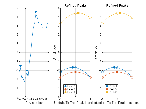
Specify the indices of the initially estimated peaks as a three-column matrix and refine the peaks across rows. Plot the estimated and refined peaks.
ax12 = nexttile;
xPeaks2D = [0 jPks kPks] + [1 0 0].*iPks;
refinepeaks(temps3D,xPeaks2D)
subtitle(["Location Indices:";"Numeric Matrix"])
Define a logical array specifying a value of true at the indices of the initially estimated peaks. Specify the logical array as the peak location index input to refine the peaks. Plot the refined peaks. Whether you specify the location indices of the initially estimated peaks as a numeric matrix or a logical array, the result is the same.
ax13 = nexttile;
xPeaks3D = false(size(temps3D));
xPeaks3D(iPks,jPks,kPks) = true; % Logical indices
refinepeaks(temps3D,xPeaks3D) % Refined peaks
subtitle(["Location Indices:";"Logical Array"])
linkaxes([ax11 ax12 ax13],"y")
Peaks Across Weekdays (Columns)
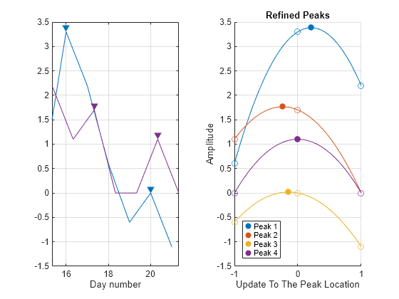
Find the temperature peaks at midnight and at 8 a.m. along all weekdays of the third week. Estimate the peak amplitudes and locations. Specify a logical array of initially estimated peaks and refine the peaks across columns. Plot the estimated and refined peaks.
iPks1 = 1;
iPks2 = 9;
kPks = 3;
[EstPks1,jPks1] = findpeaks(temps3D(iPks1,:,kPks));
[EstPks2,jPks2] = findpeaks(temps3D(iPks2,:,kPks));

tiledlayout("horizontal")
ax21 = nexttile;
findpeaks(temps3D(iPks1,:,kPks),times3D(iPks1,:,kPks))
text(times3D(iPks1,jPks1,kPks)+.02,EstPks1,string((1:numel(EstPks1))'))
hold on
findpeaks(temps3D(iPks2,:,kPks),times3D(iPks2,:,kPks))
text(times3D(iPks2,jPks2,kPks)+.02,EstPks2, ...
    string(numel(EstPks1)+(1:numel(EstPks2))'))
hold off
legend(["12 a.m." "" "8 a.m."])
xlabel("Day Number")
ylabel("Amplitude")
title("Estimated Peaks")

ax22 = nexttile;
xPeaks3D = false(size(temps3D));
xPeaks3D(iPks1,jPks1,kPks) = true;
xPeaks3D(iPks2,jPks2,kPks) = true;
refinepeaks(temps3D,xPeaks3D,Dimension=2)
subtitle("Location Indices: Logical Array")
linkaxes([ax21 ax22],"y")
Peaks Across Weeks (Pages)
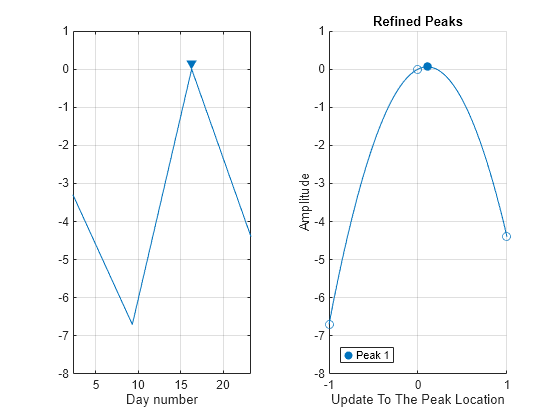
Find the temperature peaks at 7 a.m. during the second day of all weeks. Estimate the peak amplitudes and locations. Specify the indices of the initially estimated peaks as a three-column matrix and refine the peaks across pages. Plot the estimated and refined peaks.
iPks = 8;
jPks = 2;
tempsD27am = temps3D(iPks,jPks,:);
timesD27am = times3D(iPks,jPks,:);
[EstPks,kPks] = findpeaks(tempsD27am(:));

tiledlayout("horizontal")
ax31 = nexttile;
findpeaks(tempsD27am(:),timesD27am(:));
text(times3D(iPks,jPks,kPks)+0.02,EstPks,string((1:numel(EstPks))'))
xlabel("Day Number")
ylabel("Amplitude")
title("Estimated Peaks")

ax32 = nexttile;
xPeaks2D = [iPks jPks 0] + [0 0 1].*kPks;
refinepeaks(temps3D,xPeaks2D,Dimension=3)
subtitle("Location Indices: Numeric Matrix")
linkaxes([ax31 ax32],"y")

Input Arguments
Signal amplitude data, specified as a real-valued vector, matrix,
N-dimensional array, or MATLAB® timetable with one- or two-dimensional data representing the input signal
amplitudes. You must specify y so its representing data contains at
least a three-element vector. The refinepeaks function uses three
points to refine each peak: the selected peak and two surrounding points.
Example: y = [100 77; 98.7 82.6; 95.2 86.5; 101.4 84.7; 99.1 84.3]
specifies a matrix representing two five-element signal amplitude
vectors.
Example: y = timetable([100;98.7;95.2;101.4;99.1],SampleRate=100)
specifies a timetable with one-dimensional data represented by a five-element column
vector.
Data Types: single | double | timetable
Location indices of the initially estimated peaks, specified as one of the following:
Scalar, vector or matrix of positive integers — The function assumes that
xPeaksIdxrepresents the location indices of the initial peak estimates ofy. The dimensionality ofxPeaksIdxdepends on how you specifyy.If you specify
yas a vector or timetable with one-column data,xPeaksIdxmust be either a scalar representing the index of one peak or a vector representing the indices of multiple peaks.If you specify
yas a matrix or as an N-dimensional array,xPeaksIdxmust be either a row vector representing the index of one peak or a two-dimensional matrix representing the indices of multiple peaks.
xPeaksIdxmust be of size of M-by-N, wherexPeaksIdxpoints at the indices of the M peaks of interest in the N-dimensional inputy.N-dimensional array of logical values with the same size as
y— The function assumes that any location index inxPeaksIdxwith a logical value of1(true) points to a peak iny.
If any element of xPeaksIdx that you specify selects the first
or last element of y for the Dimension of
interest, or if it selects a value that is not a peak, then
refinepeaks does not perform peak processing. Instead,
refinepeaks returns the same original (unrefined) peak values and
locations in yRPeaks and xRPeaks,
respectively.
Example: xPeaksIdx = 4 specifies that the fourth sample of a
vector y is an initially estimated peak.
Example: xPeaksIdx = [4 1; 7 6; 5 8] specifies three peaks to
refine: the fourth sample of the first column of y, the seventh
sample of the sixth column of y, and the fifth sample of the eighth
column of y.
Data Types: single | double | logical
Scaled locations of the signal amplitude data, specified as a real-valued,
datetime, or duration vector.
The vector
xmust increase or decrease monotonically and uniformly. It must also have the same length as the number of elements inyalong theDimensionof interest.If you do not specify
x,refinepeaksgeneratesxfrom the indices ofyalong theDimensionof interest. In other words,refinepeakssetsxto the vector1:Q, whereQis the number of samples inyalong theDimensionof interest.You cannot specify
xif you specifyyas a timetable. When you specifyyas a timetable,refinepeaksassigns the time values fromytox.
The refinepeaks function uses x
to adjust xRPeaks to match the desired signal scale.
xRPeaks can represent time, frequency, angle, or any other
metric.
Example: x = seconds(0:0.01:1) specifies the
duration locations of the signal amplitude data points in a 101-element
vector y. If you do not specify x,
refinepeaks assumes x = 1:101, given the same
vector y.
Example: x = 501:699 specifies the locations of the signal
amplitude data points in an N-D array y with 200
samples across the dimension of interest. If you do not specify x,
refinepeaks assumes x = 1:200, given the same
N-D array y.
Data Types: single | double | datetime | duration
Name-Value Arguments
Specify optional pairs of arguments as
Name1=Value1,...,NameN=ValueN, where Name is
the argument name and Value is the corresponding value.
Name-value arguments must appear after other arguments, but the order of the
pairs does not matter.
Example: [yRPeaks,xRPeaks] =
refinepeaks(y,xPeaksIdx,x,Dimension=2,Method="NLS",MaxIterations=7) refines
the peaks with locations in xPeaksIdx across the second dimension of
the N-D array y using scaled locations
x, the nonlinear squares (NLS) method, and seven iterations at
maximum.
Peak Refinement
Peak refinement method, specified as one of these values:
"QLS"—refinepeaksuses the quadratic least squares (QLS) method to refine the peaks, representing each peak and the corresponding two surrounding points with a curve-fitting quadratic function. See QLS Method for additional input arguments."NLS"—refinepeaksuses the nonlinear least squares (NLS) fractional peak estimation method, representing each peak and the corresponding two surrounding points with a curve-fitting sinc function. Therefinepeaksfunction uses the Gauss-Newton implementation and a sinc-function kernel to perform the curve-fitting operation. See NLS Method for additional input arguments.
For more information about these peak refinement methods, see Algorithms.
Data Types: char | string
Dimension along which to refine the peaks in y, specified as
a positive integer scalar.
If you specify
yas an N-dimensional matrix,Dimensionmust be an integer scalar between 1 and N.If you do not specify
Dimension,refinepeakssets the value to the first dimension with at least three elements. For example, if you specify a signal with amplitudesyof size 2-by-1-by-2-by-6-by-7,refinepeakssetsDimensionto4.
Assume an N-dimensional array y of size [s1
s2 ⋯
sn – 1
sn
sn + 1 ⋯
sN – 1
sN] and you intend to refine peaks across the nth
dimension. When you specify Dimension=n,
refinepeaks refines each peak of y
assuming the following location indices.
| Sample | Location index |
|---|---|
| Peak |
[p1 p2 ⋯ pn – 1 pn pn + 1 ⋯ pN – 1 pN] |
| Left surrounding |
[p1 p2 ⋯ pn – 1 pn–1 pn + 1 ⋯ pN – 1 pN] |
| Right surrounding |
[p1 p2 ⋯ pn – 1 pn+1 pn + 1 ⋯ pN – 1 pN] |
Data Types: single | double
QLS Method
Amplitude preprocessing kernel for the QLS method, specified as one of these values:
"none"—refinepeaksusesyto refine peaks."log"—refinepeaksuseslog10(y)to refine peaks."exp"—refinepeaksusesy.^kto refine peaks, wherekis the exponent specified inKernelPower.
Dependencies
You must set Method to "QLS" to
specify QLSKernel.
Data Types: char | string
Exponent of the exponential QLS kernel, specified as a positive scalar.
Dependencies
You must set QLSKernel to "exp" to
specify KernelPower.
Data Types: single | double
NLS Method
Width of the interpolating sinc curves where the peaks reside, specified as a
scalar or column vector with as many rows as peaks you specified to refine in
xPeaksIdx. The minimum value of LobeWidth
must be equal or greater than 2.
LobeWidthrepresents the estimate of the width of the lobes where the selected peaks are located in terms of number of samples.If you specify
LobeWidthas a scalar,refinepeaksapplies the same lobe width to all the peak location entries inxPeaksIdx.If you specify
LobeWidthas a column vector,refinepeaksapplies the lobe width from each row ofLobeWidthto its corresponding peak location entry inxPeaksIdx.
The
refinepeaksfunction usesLobeWidthas an initial estimate for the function kernel in the iterative computation.You can obtain an initial estimate of
LobeWidthfrom the initially estimated peaks usingfindpeaksfunction. See Tips for more information.Although you do not need to specify exact values for
LobeWidth, a good initial estimate can help the NLS method converge faster. Conversely, if the values inLobeWidthare far from the actual values, the NLS method might not converge to the correct values.
Dependencies
You must set Method to "NLS" to
specify LobeWidth.
Data Types: single | double
Maximum number of iterations, specified as a positive integer scalar greater than or equal to 3. For more information about the iteration process, see Peak Iterative Refinement.
Generally, between 5 and 10 iterations are needed to reach the final refined peak estimates.
Dependencies
You must set Method to "NLS" to
specify MaxIterations.
Data Types: single | double
Maximum squared error threshold, specified as a positive scalar.
SquaredErrorThreshold represents the threshold tolerance for
the sum of squared differences in amplitude between each three-point set (peak and two
surroundings) from y and the corresponding amplitude evaluation
of the refined curve of y that refinepeaks
fits using the NLS method.
For more information about the iteration process, see Peak Iterative Refinement.
Dependencies
You must set Method to "NLS" to
specify MaxIterations.
Data Types: single | double
Output Arguments
Tips
You can initially estimate signal peaks with findpeaks, and then enhance their amplitudes and locations with
refinepeaks.
Assume you have a signal with amplitudes y and locations
x. The following code snippet shows how you can estimate and refine
peaks from y and x.
[yPeaks,xPeaksIdx] = findpeaks(y);
[yRPeaks,xRPeaks] = refinepeaks(y,xPeaksIdx,x)
Add name-value arguments for further customization. For example, you can specify
LobeWidth from the width of the initially estimated
peaks.
[yPeaks,xPeaksIdx,xWidths] = findpeaks(y);
[yRPeaks,xRPeaks] = refinepeaks(y,xPeaksIdx,x,Method="NLS", ...
    LobeWidth=max(xWidths,2))
Algorithms
For each selected peak with location index xPI
from the vector of indices xPeaksIdx, refinepeaks
identifies the indices and amplitudes of the peak y1
and its two surrounding points y0 and
y2 from y along
Dimension. These three samples form the vector Y such that
The refinepeaks function uses the quadratic least square (QLS) or
nonlinear least square (NLS) fractional peak estimation algorithm to refine initially
estimated peaks from signal amplitude data.
The QLS algorithm [2] preprocesses the signal amplitudes of Y, refines the peak location index by fitting and differentiating a quadratic polynomial, and then calculates the refined peak amplitude and scaled location.
Unless you specify QLSKernel as "none", in
which case refinepeaks skips the data preprocessing step, the QLS
algorithm starts by preprocessing the signal amplitude data Y using the QLSKernel that you specify. While
logarithmic preprocessing ("log" QLS kernel) is commonly used for
phased and radar applications, exponential preprocessing ("exp" QLS
kernel) is used in other signal applications.
The function transforms the signal amplitudes of the peak and surrounding points for peak refinement, such that y0, y1, and y2 have these values:
| Logarithmic Processing | Exponential Processing |
|---|---|
|
y0 = log10|y[xPI – 1]| |
y0 = |y[xPI – 1]|k |
|
y1 = log10|y[xPI]| |
y1 = |y[xPI]|k |
|
y2 = log10|y[xPI + 1]| |
y2 = |y[xPI + 1]|k |
For logarithmic processing, specify the exponentk using
KernelPower.
The function refines the peak location index by performing quadratic least square estimation using y0, y1, and y2 and differentiates the least-square quadratic polynomial to obtain a subsample estimate of the peak location, xRPI, where
The function reverts the values of y0, y1, and y2 to their original values before preprocessing.
The function calculates the scaled location of the refined peak
xRPeak from
xRPI and from the scaled locations of signal
amplitude data x, if you specify one.
If you specify the scaled locations of signal amplitude data
x, then the function scales xRPI for each peak and sets each element ofxRPeaksfrom xRP, such thatwhere x0 = x[xRPI − 1], x1 = x[xRPI], and x2 = x[xRPI + 1].
If you do not specify
x, then the function sets each element ofxRPeakssuch that xRPeak = xRPI.
The function calculates the refined peak amplitude yRPeak from the least-square quadratic polynomial such that
where a = (y0 – 2y1 + y2)/2, b = (y2 – y0)/2, and c = y1.
The NLS algorithm [4] uses a sinc-function kernel to fit the curve formed by the initially estimated peak and its two surrounding points, followed by an minimum-error optimization, and then calculates the refined peak amplitude.
Assume the function f(X;λ) depends on the input column vector X and on the curve-fitting parameter vector λ such that f produces the column vector Y.
where X = [–1 0 1]T and λ = [λ0 λ1 λ2]T.
The refinepeaks function estimates the parameter vector λ to refine the peak location and amplitude such that λ minimizes the residual error S,
The refinepeaks function uses Gauss–Newton optimization, for
which it finds the gradients with respect to λ0,
λ1, and
λ2 such that
Then, refinepeaks performs the optimization as an
iterative process, with initial parameter values λ0 =
|y[xPI]|, λ1 =
eps, and λ2 =
1/LW, where LW is the peak width specified in LobeWidth.
At the mth iteration, where m varies from 1 to
MaxIterations, the function calculates the Jacobian matrix J and the residual error vector ΔY.
Since JΔλ = ΔY, solving the equation system derives in the calculation of the variation of the parameter vector λ such that
The function calculates the residual error S for the mth iteration from the squared sum of the elements in ΔY.
The iteration process stops as soon as one of these occurs:
The
MaxIterations-th iteration is complete.The residual error S is less or equal to
SquaredErrorThreshold.
The refinepeaks function first calculates the subsample estimate
of the peak location xRPI using the final value
of λ1 from the Peak Iterative Refinement process, where
Then, refinepeaks calculates the scaled location of the refined
peak xRPeak from
xRPI and from the scaled locations of signal
amplitude data x, if you specify one.
If you specify the scaled locations of signal amplitude data
x, then the function scales xRPI for each peak and sets each element ofxRPeaksfrom xRP such thatwhere x0 = x[xRPI − 1], x1 = x[xRPI], and x2 = x[xRPI + 1].
If you do not specify
x, then the function sets each element ofxRPeakssuch that xRPeak = xRPI.
The refinepeaks function calculates the refined peak amplitude
yRPeak from the fitted sinc function such that
where the coefficients λ0, λ1, and λ2 are the final values from the Peak Iterative Refinement process.
References
[1] Richards, Mark A., James A. Scheer, and William A. Holm, eds. Principles of Modern Radar: Basic Principles. Institution of Engineering and Technology, 2010.
[2] Moddemeijer, R. “On the Determination of the Position of Extrema of Sampled Correlators.” IEEE® Transactions on Signal Processing 39, no. 1 (January 1991): 216–19.
[3] Sharp, I., K. Yu, and Y. J. Guo. “Peak and Leading Edge Detection for Time-of-Arrival Estimation in Band-Limited Positioning Systems.” IET Communications 3, no. 10 (October 1, 2009): 1616–27.
[4] Prager, Samuel, Mark S. Haynes, and Mahta Moghaddam. “Wireless Subnanosecond RF Synchronization for Distributed Ultrawideband Software-Defined Radar Networks.” IEEE Transactions on Microwave Theory and Techniques 68, no. 11 (November 2020): 4787–4804.
Extended Capabilities
C/C++ Code Generation
Generate C and C++ code using MATLAB® Coder™.
GPU Code Generation
Generate CUDA® code for NVIDIA® GPUs using GPU Coder™.
Version History
Introduced in R2024b
See Also
findpeaks | islocalmax | max
MATLAB Command
You clicked a link that corresponds to this MATLAB command:
Run the command by entering it in the MATLAB Command Window. Web browsers do not support MATLAB commands.
Select a Web Site
Choose a web site to get translated content where available and see local events and offers. Based on your location, we recommend that you select: .
You can also select a web site from the following list
How to Get Best Site Performance
Select the China site (in Chinese or English) for best site performance. Other MathWorks country sites are not optimized for visits from your location.
Americas
- América Latina (Español)
- Canada (English)
- United States (English)
Europe
- Belgium (English)
- Denmark (English)
- Deutschland (Deutsch)
- España (Español)
- Finland (English)
- France (Français)
- Ireland (English)
- Italia (Italiano)
- Luxembourg (English)
- Netherlands (English)
- Norway (English)
- Österreich (Deutsch)
- Portugal (English)
- Sweden (English)
- Switzerland
- United Kingdom (English)