invfreqz

Identify discrete-time filter parameters from frequency response data

Syntax

[b,a] = invfreqz(h,w,n,m)

[b,a] = invfreqz(h,w,n,m,wt)

[b,a] = invfreqz(___,iter)

[b,a] = invfreqz(___,tol)

[b,a] = invfreqz(___,'trace')

[b,a] = invfreqz(h,w,'complex',n,m,___)

Description

[b,a] = invfreqz(h,w,n,m) returns the real numerator and denominator coefficient vectors b and a of the transfer function h.

[b,a] = invfreqz(h,w,n,m,wt) weights the fit-errors versus frequency using wt.

[b,a] = invfreqz(___,iter) provides an algorithm that guarantees stability of the resulting linear system by searching for the best fit using a numerical, iterative scheme. This syntax can include any combination of input arguments from the previous syntaxes.

[b,a] = invfreqz(___,tol) uses tol to decide convergence of the iterative algorithm.

[b,a] = invfreqz(___,'trace') displays a textual progress report of the iteration.

[b,a] = invfreqz(h,w,'complex',n,m,___) creates a complex filter. In this case no symmetry is enforced, and the frequency is specified in radians between –π and π.

Examples

Stable Approximate Transfer Function

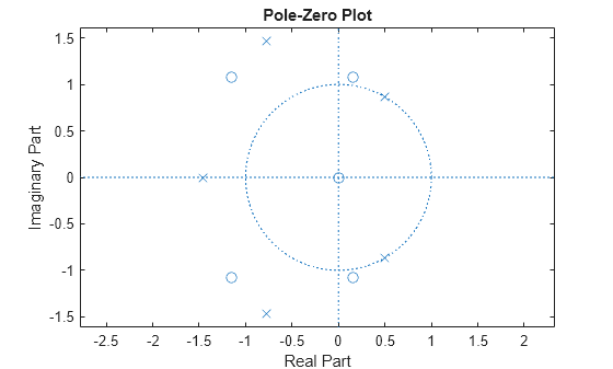
Convert a simple transfer function to frequency response data and then back to the original filter coefficients. Sketch the zeros and poles of the function.

a = [1 2 3 2 1 4];
b = [1 2 3 2 3];

[h,w] = freqz(b,a,64);
[bb,aa] = invfreqz(h,w,4,5)

bb = 1×5 complex

   1.0000 + 0.0000i   2.0000 + 0.0000i   3.0000 + 0.0000i   2.0000 + 0.0000i   3.0000 + 0.0000i

aa = 1×6

    1.0000    2.0000    3.0000    2.0000    1.0000    4.0000

zplane(bb,aa)

bb and aa are equivalent to b and a, respectively. However, the system is unstable because it has poles outside the unit circle. Use invfreqz's iterative algorithm to find a stable approximation to the system. Verify that the poles are within the unit circle.

[bbb,aaa] = invfreqz(h,w,4,5,[],30)

  INITIAL ESTIMATE
Current fit: 4806.3373
par-vector
    0.2500
    0.5000
    0.7500
    0.5000
    0.2500
    1.0000
    2.0000
    3.0000
    2.0000
    3.0000

0
      ITERATION # 1
Current fit:  19.1832  Previous fit:  4806.3373
Current par prev.par   GN-dir
    0.2490    0.2500    0.0015
    0.4941    0.5000    0.0055
    0.7536    0.7500   -0.0045
    0.4944    0.5000    0.0050
    0.2480    0.2500    0.0017
    0.2404    1.0000    0.7596
    0.5538    2.0000    1.4462
    0.5149    3.0000    2.4851
    0.2497    2.0000    1.7503
    0.0749    3.0000    2.9251

Norm of GN-vector: 4.5237
0
1
      ITERATION # 2
Current fit:  18.8642  Previous fit:  19.1832
Current par prev.par   GN-dir
   -0.5984    0.2490    1.6948
    0.3132    0.4941    0.3619
    0.7897    0.7536   -0.0723
   -0.3866    0.4944    1.7620
    0.1039    0.2480    0.2883
    0.2406    0.2404   -0.0004
    0.3507    0.5538    0.4061
    0.0559    0.5149    0.9181
   -0.0596    0.2497    0.6186
    0.0415    0.0749    0.0669

Norm of GN-vector: 2.7552
0
1
2
      ITERATION # 3
Current fit:  18.475  Previous fit:  18.8642
Current par prev.par   GN-dir
   -0.7672   -0.5984    0.6761
    0.5640    0.3132   -1.0049
    0.9052    0.7897   -0.4623
   -0.6713   -0.3866    1.1395
    0.4694    0.1039   -1.4627
    0.2410    0.2406   -0.0018
    0.3106    0.3507    0.1604
    0.0346    0.0559    0.0851
    0.0466   -0.0596   -0.4247
    0.1378    0.0415   -0.3853

Norm of GN-vector: 2.341
0
1
2
3
      ITERATION # 4
Current fit:  18.1494  Previous fit:  18.475
Current par prev.par   GN-dir
   -0.8883   -0.7672    0.9702
    0.6817    0.5640   -0.9440
    0.9919    0.9052   -0.6941
   -0.8794   -0.6713    1.6657
    0.6735    0.4694   -1.6347
    0.2418    0.2410   -0.0065
    0.2805    0.3106    0.2409
    0.0042    0.0346    0.2438
    0.0920    0.0466   -0.3634
    0.1908    0.1378   -0.4242

Norm of GN-vector: 2.8619
0
1
2
3
4
5
6
      ITERATION # 5
Current fit:  18.1371  Previous fit:  18.1494
Current par prev.par   GN-dir
   -0.8938   -0.8883    0.0268
    0.6934    0.6817   -0.1305
    0.9938    0.9919   -0.9589
   -0.8868   -0.8794    0.9873
    0.6870    0.6735   -1.0885
    0.2424    0.2418   -0.0355
    0.2794    0.2805    0.0735
    0.0059    0.0042   -0.1113
    0.0954    0.0920   -0.2197
    0.1957    0.1908   -0.3106

Norm of GN-vector: 1.8057
0
1
2
3
4
5
6
7
      ITERATION # 6
Current fit:  18.0937  Previous fit:  18.1371
Current par prev.par   GN-dir
   -0.8944   -0.8938    0.0134
    0.6954    0.6934   -0.1440
    0.9997    0.9938   -0.9120
   -0.8933   -0.8868    0.9270
    0.6950    0.6870   -1.0552
    0.2427    0.2424   -0.0354
    0.2788    0.2794    0.0723
    0.0069    0.0059   -0.1234
    0.0971    0.0954   -0.2167
    0.1980    0.1957   -0.3043

Norm of GN-vector: 1.7282
0
1
2
3
4
5
6
7
8
9
10
11
12
13
14
15
16
17
      ITERATION # 7
Current fit:  18.0409  Previous fit:  18.0937
Current par prev.par   GN-dir
   -0.8944   -0.8944   -0.0007
    0.6954    0.6954   -0.0019
    0.9997    0.9997   -0.0012
   -0.8933   -0.8933    0.0006
    0.6949    0.6950    0.0018
    0.2427    0.2427   -0.0000
    0.2788    0.2788    0.0001
    0.0069    0.0069    0.0001
    0.0971    0.0971    0.0000
    0.1980    0.1980   -0.0001

Norm of GN-vector: 0.0030376

bbb = 1×5 complex

   0.2427 + 0.0000i   0.2788 + 0.0000i   0.0069 + 0.0000i   0.0971 + 0.0000i   0.1980 + 0.0000i

aaa = 1×6

    1.0000   -0.8944    0.6954    0.9997   -0.8933    0.6949

zplane(bbb,aaa)

Input Arguments

h — Frequency response

vector

Frequency response, specified as a vector.

w — Angular frequencies

vector

Angular frequencies at which h is computed, specified as a vector.

n, m — Desired order

positive integer scalar

Desired order of the numerator and denominator polynomials, specified as positive integer scalars.

wt — Weighting factors

vector

Weighting factors, specified as a vector. wt is a vector of weighting factors that is the same length as w.

iter — Number of iterations in the search algorithm

positive real scalar

Number of iterations in the search algorithm, specified as a positive real scalar. The iter parameter tells invfreqz to end the iteration when the solution has converged, or after iter iterations, whichever comes first.

tol — Tolerance

0.01 (default) | scalar

Tolerance, specified as a scalar. invfreqz defines convergence as occurring when the norm of the (modified) gradient vector is less than tol.

To obtain a weight vector of all ones, use

invfreqz(h,w,n,m,[],iter,tol)

Output Arguments

b, a — Transfer function coefficients

vectors

Transfer function coefficients, returned as vectors. Express the transfer function in terms of b and a as

$$H(z)=\frac{B(z)}{A(z)}=\frac{b_1+b_2{z}^{-1}\cdots +b_n{z}^{-\left(n-1\right)}+b_{n+1}{z}^{-n}}{a_1+a_2{z}^{-1}\cdots +a_m{z}^{-\left(m-1\right)}+a_{m+1}{z}^{-m}}$$

Example: b = [1 3 3 1]/6 and a = [3 0 1 0]/3 specify a third-order Butterworth filter with normalized 3 dB frequency 0.5π rad/sample.

Data Types: double | single
Complex Number Support: Yes

Algorithms

By default, invfreqz uses an equation error method to identify the best model from the data. The method finds b and a in

$$\underset{b,a}{\min }{\displaystyle \sum _{k=1}^{n}wt(k){\left|h(k)A(w(k))-B(w(k))\right|}^2}$$

by creating a system of linear equations and solving them with the MATLAB^® \ operator. Here A(ω(k)) and B(ω(k)) are the Fourier transforms of the polynomials a and b, respectively, at the frequency ω(k), and n is the number of frequency points (the length of h and w). This algorithm is a based on Levi [1].

The superior ("output-error") algorithm uses the damped Gauss-Newton method for iterative search [2], with the output of the first algorithm as the initial estimate. This solves the direct problem of minimizing the weighted sum of the squared error between the actual and the desired frequency response points.

$$\underset{b,a}{\min }{\displaystyle \sum _{k=1}^{n}wt(k){\left|h(k)-\frac{B(w(k))}{A(w(k))}\right|}^2}$$

References

[1] Levi, E. C. “Complex-Curve Fitting.” IRE Transactions on Automatic Control. Vol. AC-4, 1959, pp. 37–44.

[2] Dennis, J. E., Jr., and R. B. Schnabel. Numerical Methods for Unconstrained Optimization and Nonlinear Equations. Englewood Cliffs, NJ: Prentice-Hall, 1983.

Extended Capabilities

C/C++ Code Generation
Generate C and C++ code using MATLAB® Coder™.

Version History

Introduced before R2006a

R2024b: invfreqz supports C/C++ code generation

The invfreqz function supports C/C++ code generation. You must have MATLAB Coder™ to use this functionality.