FVTool

(To be removed) Filter Visualization Tool

FVTool will be removed in a future release. Use Filter Analyzer instead. For more information, see Version History.

Description

Filter Visualization Tool is an interactive app that enables you to display and analyze the responses, coefficients, and other information of a filter. You can also synchronize FVTool and Filter Designer to immediately visualize any changes made to a filter design.

In the app, you can view:

• Magnitude response

• Phase response

• Group delay

• Phase delay

• Impulse response

• Step response

• Pole-zero plot

• Filter coefficients

• Filter information

For more information, see Analysis Types.

If you have installed the DSP System Toolbox™, FVTool can also visualize the frequency response of a filter System object™. If you need to filter streaming data in real time, using System objects is the recommended approach. For more information, see fvtool (DSP System Toolbox).

Open the FVTool

FVTool can be opened programmatically using one of the methods described in Programmatic Use.

Examples

Magnitude Response of Elliptic Filter

Consider a 6th-order elliptic filter with a passband ripple of 3 dB, a stopband attenuation of 50 dB, a sample rate of 1 kHz, and a normalized passband edge of 300 Hz. Display the magnitude response of the filter.

[b,a] = ellip(6,3,50,300/500);
fvtool(b,a)

Programmatic Use

fvtool(b,a) opens FVTool and displays the magnitude response of the digital filter defined with numerator b and denominator a. Specify b and a coefficients in ascending order of power z^-1.

fvtool(sos) opens FVTool and displays the magnitude response of the digital filter defined by the L-by-6 matrix of second order sections:

$$\text{sos}=\left[\begin{array}{cccccc}{b}_{01}& b_{11}& b_{21}& 1& a_{11}& a_{21}\\ b_{02}& b_{12}& b_{22}& 1& a_{12}& a_{22}\\ ⋮& ⋮& ⋮& ⋮& ⋮& ⋮\\ b_{0L}& b_{1L}& b_{2L}& 1& a_{1L}& a_{2L}\end{array}\right]$$

The rows of sos contain the numerator and denominator coefficients b_ik and a_ik of the cascade of second-order sections of H(z):

$$H(z)=g{\displaystyle \prod _{k=1}^L{H}_k}(z)=g{\displaystyle \prod _{k=1}^L\frac{b_{0k}+b_{1k}{z}^{-1}+b_{2k}{z}^{-2}}{1+a_{1k}{z}^{-1}+a_{2k}{z}^{-2}}}.$$

The number of sections L must be greater than or equal to 2. If the number of sections is less than 2, fvtool considers the input to be a numerator vector.

fvtool(d) opens FVTool and displays the magnitude response of a digital filter d. Use designfilt to generate d based on frequency-response specifications.

fvtool(b1,a1,b2,a2,...,bN,aN) opens FVTool and displays the magnitude responses of multiple filters defined with numerators b1, …, bN and denominators a1, ..., aN.

fvtool(sos1,sos2,...,sosN) opens FVTool and displays the magnitude responses of multiple filters defined with second order section matrices sos1, sos2, ..., sosN.

fvtool(Hd) opens FVTool and displays the magnitude responses for the dfilt filter object Hd or the array of dfilt filter objects.

fvtool(Hd1,Hd2,...,HdN) opens FVTool and displays the magnitude responses of the filters in the dfilt objects Hd1, Hd2, ..., HdN.

h = fvtool(___) returns a figure handle h. You can use this handle to interact with FVTool from the command line. For more information, see Control FVTool Using MATLAB Command Line.

More About

Analysis Types

FVTool has these analysis types:

Analysis	Description
Magnitude response	To see the zero-phase response, right-click the y-axis label on the plot and select Zero-phase from the context menu. For more information, see freqz and zerophase.
Phase response	For more information, see phasez.
Magnitude response and phase response	The responses are superimposed on one another. For more information, see freqz.
Group delay	Group delay is the average delay of the filter as a function of frequency. For more information, see grpdelay.
Phase delay	Phase delay is the time delay the filter imposes on each component of the input signal. For more information, see phasedelay.
Impulse response	The impulse response is the response of the filter to an impulse input. For more information, see impz.
Step response	The step response is the response of the filter to a step input. For more information, see stepz.
Pole-zero plot	The pole-zero plot shows the pole and zero locations of the filter on the z-plane. For more information, see zplane.
Filter coefficients	The coefficients depend on the filter structure (direct-form or lattice). The app displays filter coefficients in a text box. For SOS filters, the app displays each section as a separate filter.
Filter information	The filter information includes the structure, phase, stability, and implementation cost of the filter.

Control FVTool Using GUI

Display and analyze responses of one or multiple filters using controls on the toolstrip.

• By default, the app displays the magnitude response of a filter. To change the display, select an option from the Analysis list in the Analysis section of the toolstrip.

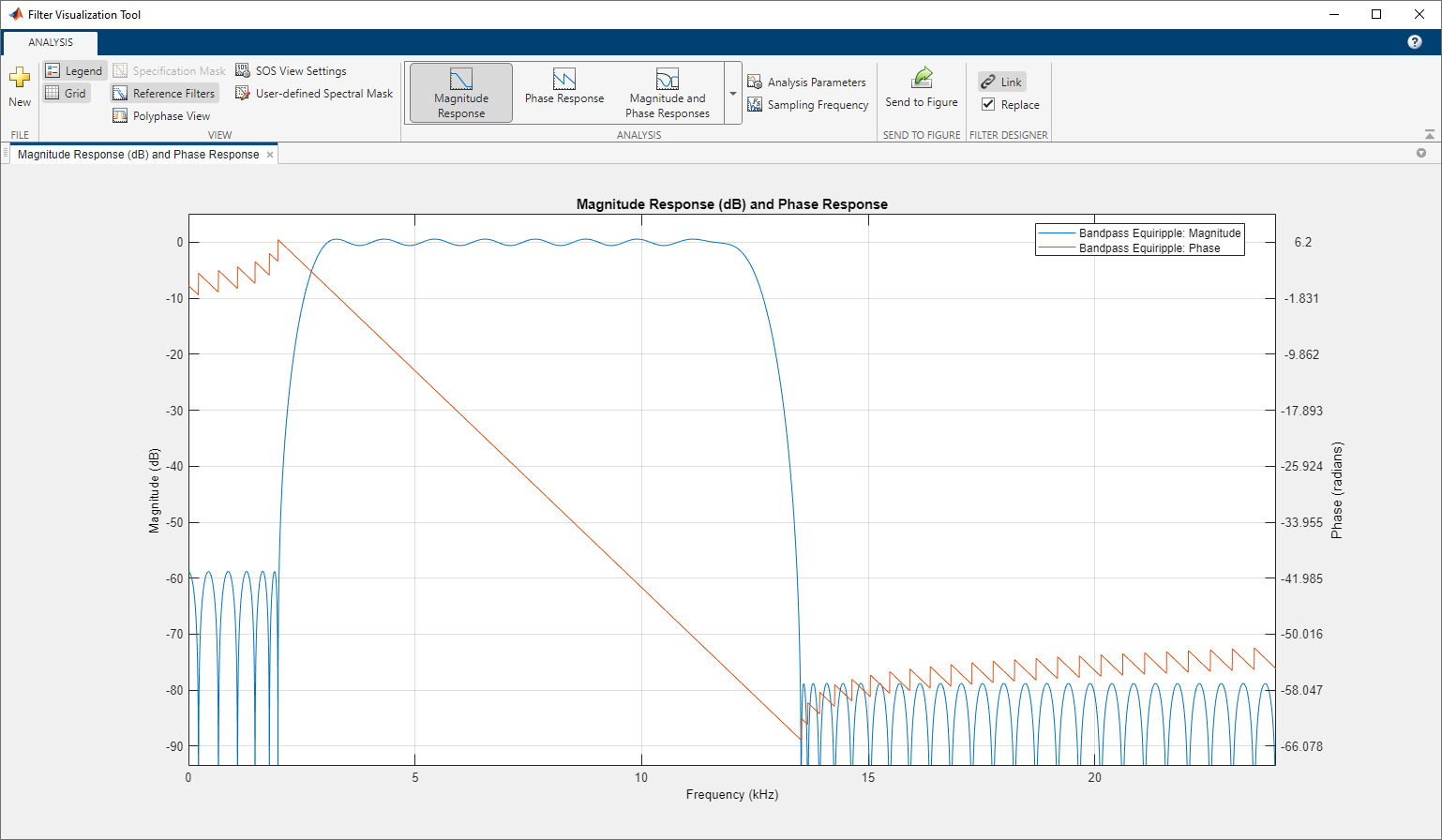
• To overlay a second response on the plot, select an available response from the Overlay Analysis list in the Analysis section of the toolstrip. The app adds a second y-axis to the right side of the response plot. The Analysis Parameters dialog box shows parameters for the x-axis and both y-axes.

• To adjust view settings, analysis parameters, or specify sampling frequency, use the corresponding buttons on the toolstrip. You can also toggle the plot legend and grid.

• To edit a plot, first click Send to Figure. In the new figure window, use the plot editing toolbar.

Control FVTool Using MATLAB Command Line

After you obtain the handle for FVTool, you can control some aspects of FVTool from the command line. In addition to the standard graphic object properties (see View List of Properties for more information), FVTool has these properties.

• Analysis — Displays the specified type of analysis plot. This table lists all analysis types and how to invoke them. Note that the only analyses that use filter internals are magnitude response estimate and round-off noise power, which are available only with DSP System Toolbox.

  Analysis Type	Analysis Option
  Magnitude plot	"magnitude"
  Phase plot	"phase"
  Magnitude and phase plot	"freq"
  Group delay plot	"grpdelay"
  Phase delay plot	"phasedelay"
  Impulse response plot	"impulse"
  Step response plot	"step"
  Pole-zero plot	"polezero"
  Filter coefficients	"coefficients"
  Filter information	"info"
  Magnitude response estimate (Available only with the DSP System Toolbox product. For more information, see freqrespest (DSP System Toolbox).)	"magestimate"
  Round-off noise power (Available only with the DSP System Toolbox product. For more information, see noisepsd (DSP System Toolbox).)	"noisepower"

• Grid — Controls whether the grid is "on" or "off".

• Legend — Controls whether the legend is "on" or "off".

• Fs — Controls the sampling frequency of filters in FVTool. The sampling frequency vector must be of the same length as the number of filters or a scalar value. If it is a vector, FVTool applies each value to its corresponding filter. If it is a scalar, FVTool applies the same value to all filters.

• SosViewSettings — (This option is available only if you have the DSP System Toolbox product.) For second-order sections filters, this controls how the filter is displayed. The SOSViewSettings property contains an object so you must use this syntax to set it: set(h.SOSViewSettings,View=viewtype), where viewtype is one of these:

  • Complete — Displays the complete response of the overall filter.

  • Individual — Displays the response of each section separately.

  • Cumulative — Displays the response for each section accumulated with each prior section. If your filter has three sections, the first plot shows section one, the second plot shows the accumulation of sections one and two, and the third plot show the accumulation of all three sections.

    You can also specify secondary scaling, which determines where the sections should be split. The secondary scaling points are the scaling locations between the recursive and the nonrecursive parts of the section. By default, the display does not use secondary scaling. To turn on secondary scaling, use this syntax. set(h.SOSViewSettings,View="Cumulative",SecondaryScaling=true)

  • UserDefined — Allows you to define which sections to display and the order in which to display them. Enter a cell array where each section is represented by its index. If you enter one index, only that section is plotted. If you enter a range of indices, the combined response of that range of sections is plotted. For example, if your filter has four sections, entering {1:4} plots the combined response for all four sections, and entering {1,2,3,4} plots the response for each section individually.

Note

You can change other properties of FVTool from the command line using the set function. Use get(h) to view property tags and current property settings.

You can use these methods with the FVTool handle:

• addfilter(h,filtobj) adds a new filter to FVTool. The new filter, filtobj, must be a dfilt filter object. You can specify the sampling frequency of the new filter with addfilter(h,filtobj,Fs=10).

• setfilter(h,filtobj) replaces the filter in FVTool with the filter specified in filtobj. You can set the sampling frequency as described above.

• deletefilter(h,index) deletes the filter at the FVTool cell array index location.

• legend(h,str1,str2,...) creates a legend in FVTool by associating str1 with filter 1, str2 with filter 2, etc. For more information, see legend.

Modify Axes

You can change the x- or y-axis units by right-clicking the mouse on the axis label or by right-clicking on the plot and selecting Analysis Parameters.

Plot	X-Axis Units	Y-Axis Units
Magnitude	Normalized Frequency Linear Frequency	Magnitude Magnitude (dB) Magnitude squared Zero-Phase
Phase	Normalized Frequency Linear Frequency	Phase Continuous Phase Degrees Radians
Magnitude and Phase	Normalized Frequency Linear Frequency	(y-axis on left side) Magnitude Magnitude (dB) Magnitude squared Zero-Phase (y-axis on right side) Phase Continuous Phase Degrees Radians
Group Delay	Normalized Frequency Linear Frequency	Samples Time
Phase Delay	Normalized Frequency Linear Frequency	Degrees Radians
Impulse Response	Samples Time	Amplitude
Step Response	Samples Time	Amplitude
Pole-Zero	Real Part	Imaginary Part

Modify Plot

In FVTool, you can interactively change view settings, set analysis parameters, and specify sampling frequency for the displayed analysis. In the toolstrip, select an option from the View or Analysis sections. You can also access the analysis parameters and sampling frequency menus by right-clicking on the plot.

To change the properties of a plot, first click the Send to Figure button in the toolstrip to open a new figure window and then use any of the buttons in the plot editing toolbar.

Analysis Parameters contains parameter settings applicable to the displayed analysis. If more than one analysis is displayed, FVTool shows only the parameters specific to the current plot. You can modify any of these parameter settings.

• Normalized Frequency — Check the box to normalize the frequency between 0 and 1. If not checked, the frequency is in hertz.

• Frequency Scale — Set the frequency scale of the y-axis scale to Linear or Log.

• Frequency Range — Set the range of the frequency axis or select Specify freq. vector to specify a frequency vector.

• Number of Points — Specify the number of samples to use to compute the response.

• Frequency Vector — Specify the frequency vector to use for plotting, if Specify freq. vector is selected in Frequency Range.

• Magnitude Display — Set they-axis units for magnitude to Magnitude, Magnitude (dB), Magnitude squared, or Zero-Phase.

• Phase Units — Set the y-axis units for phase to Degrees or Radians.

• Phase Display — Specify the type of phase plot as Phase or Continuous Phase.

• Group Delay Units — Set they-axis units for group delay to Samples or Time.

• Specify Length — Specify the length of the impulse or step response as Default or Specified.

• Length — Specify the number of points to use for the impulse or step response.

Note

Not all of these analysis fields are available for all types of plots.

In addition to these analysis parameters, you can

• change the plot type for the Impulse Response and Step Response plots by right-clicking and selecting Line with Marker, Stem or Line from the context menu.

• change the x-axis units by right-clicking the x-axis label and selecting Samples or Time.

• save the displayed parameters as the default values to use when Filter Designer or FVTool is opened by clicking Save as Default. To restore the default values, click Restore Original Defaults.

• display information about a particular point in the plot. For more information on data tips, see Interactively Explore and Analyze Plotted Data.

• zoom to the passband region. To use passband zoom, your filter must have been designed using fdesign. Passband zoom is not provided for cascaded integrator-comb (CIC) filters because CICs do not have conventional passbands.

Note

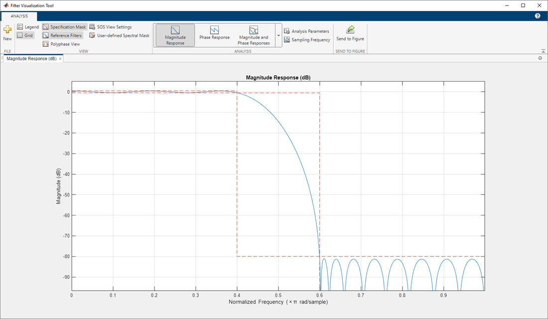
If you have a DSP System Toolbox license, FVTool displays a specification mask along with your designed filter on a magnitude plot.

Version History

Introduced before R2006a

R2026a: Warns

FVTool issues a warning that it will be removed in a future release.

R2024b: FVTool will be removed

FVTool will be removed in a future release. Use Filter Analyzer instead. There are differences that require updates to your code.

Consider these filters:

[b,a] = ellip(5,5,60,[0.2 0.45]);
dFd = designfilt("bandpassfir", ...
    SampleRate=2e3,PassbandRipple=5, ...
    StopbandFrequency1=500,PassbandFrequency1=600, ...
    StopbandAttenuation1=80, ...
    PassbandFrequency2=750,StopbandFrequency2=900, ...
    StopbandAttenuation2=40);

Given the filter numerator coefficients b, denominator coefficients a, and the digitalFilter object dFd, you must make the following updates to your code.

Original Code in R2024a or Earlier	Updated Code in R2024b
fvtool(b,a,dFd)	filterAnalyzer(b,a,dFd)
fvtool(b,a,dFd,Analysis="freq")	filterAnalyzer(b,a,dFd, ... Analysis="magnitude",Overlay="phase")
fvtool(b,a,Fs=1000)	filterAnalyzer(b,a,SampleRates=1000)
fvtool(b,a,dFd,NumberofPoints=512, ... FrequencyRange="[0, 2pi)",FrequencyScale="Log")	filterAnalyzer(b,a,dFd,NFFT=512, ... FrequencyRange="twosided",FrequencyScale="log")
hfvt = fvtool(dFd); addfilter(hfvt,dfilt.df1(b,a))	fa = filterAnalyzer(dFd); addFilters(fa,b,a)
hfvt = fvtool(dFd); setfilter(hfvt,dfilt.df1(b,a))	fa = filterAnalyzer(dFd,FilterNames="df"); replaceFilters(fa,b,a,FilterNames="df")
hfvt = fvtool(b,a,dFd); deletefilter(hfvt,2)	fa = filterAnalyzer(b,a,dFd,FilterNames=["ba" "dFd"]); deleteFilters(fa,FilterNames="dFd")
hfvt = fvtool(b,a,dFd); legend(hfvt,"ba","dFd")	filterAnalyzer(b,a,dFd,FilterNames=["ba" "dFd"])
hfvt = fvtool(b,a,dFd); zoom(hfvt,[0.4 0.7 -30 0])	fa = filterAnalyzer(b,a,dFd); zoom(fa,"xy",[0.4 0.7 -30 0])
fvtool(b,a,dFd,Analysis="noisepower")	filterAnalyzer(b,a,dFd,Analysis="noisepsd")

The second order sections (SOS) format is not supported in Filter Analyzer. Use the Cascaded Transfer Functions format instead. Given a filter specified as an SOS matrix sos, you must make the following updates to your code.

Original Code in R2024a or Earlier	Updated Code in R2024b
fvtool(sos)	filterAnalyzer(sos(:,1:3),sos(:,4:6)) or [ctfNum,ctfDen] = sos2ctf(sos); filterAnalyzer(ctfNum,ctfDen)
hfvt = fvtool(sos); set(hfvt.SOSViewSettings,View="cumulative")	[ctfNum,ctfDen] = sos2ctf(sos); fa = filterAnalyzer(ctfNum,ctfDen,CTFAnalysisMode="cumulative");
hfvt = fvtool(sos); set(hfvt.SOSViewSettings,View="userdefined",UserDefined={3,1})	[ctfNum,ctfDen] = sos2ctf(sos); fa = filterAnalyzer(ctfNum,ctfDen, ... CTFAnalysisMode="specify",CTFAnalysisSections={3,1});

R2022a: Controls are on the toolstrip

The behavior of FVTool has changed. In previous releases, the app had plot editing and analysis toolbars. Starting this release, access filter visualization controls on the toolstrip. To edit a plot, first export the plot to a figure and then use the figure controls.