Surrogate Optimization and Scripting for SerDes System Design

This example shows how to use surrogate optimization and MATLAB® scripting to automatically design and tune a SerDes system. To illustrate these concepts, consider the task of maximizing the area of the statistical eye of a SerDes system that consists of a feed-forward equalizer (FFE) in the transmitter (Tx) and a decision feedback equalizer (DFE) in the receiver (Rx). To achieve this goal, this example uses a surrogate-based method to optimize the tap weights of the FFE and the DFE. The workflow entails the following steps.

1. Create the initial architecture of the SerDes system using the SerDes Designer app in SerDes Toolbox™.

2. Export the SerDes system from the app to a MATLAB script.

3. Create an optimization objective function from the exported script.

4. Use the surrogateopt function from Global Optimization Toolbox™ to determine the optimal Tx FFE and Rx DFE tap weights.

5. Validate the optimized design by examining the pulse response, eye diagram, and other performance metrics.

Surrogate optimization is a technique for global optimization that is especially well-suited for time-consuming objective functions. As such, it is a popular choice for design optimization tasks in which the design variable space has finite, well-defined bounds. The algorithm involves iteratively constructing and training surrogate models to approximate the objective function and using these surrogates to drive the optimization search trajectory while minimizing the number of evaluations of the actual objective function. From a time perspective, the surrogate models are inexpensive to evaluate, enabling the optimizer to perform wide searches more quickly in search of a global optimum. For more information, refer to the following links:

• Surrogate Optimization

• What Is Surrogate Optimization? (Global Optimization Toolbox)

Set Up Initial Architecture of SerDes System

Create Default SerDes System

Launch the SerDes Designer app using the following command.

serdesDesigner

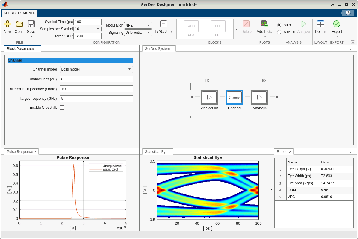
The default SerDes system contains a transmitter with an AnalogOut block, a channel, and a receiver with an AnalogIn block. By default, the simulation of the blocks in the system is configured to process the signals as differential with a symbol time of 100 ps, 16 samples per symbol, a target bit error rate (BER) of 1e-6, and a non-return-to-zero (NRZ) modulation scheme.

Evaluate Initial System Performance

Use the options in Add Plots in the SerDes Designer app toolstrip to examine the Pulse Response, Statistical Eye, and Report containing the key metrics. In the Pulse Response plot, zoom in along the time axis to the range [0,5e-9] to better visualize the pulse response.

Add 2-Tap Tx FFE

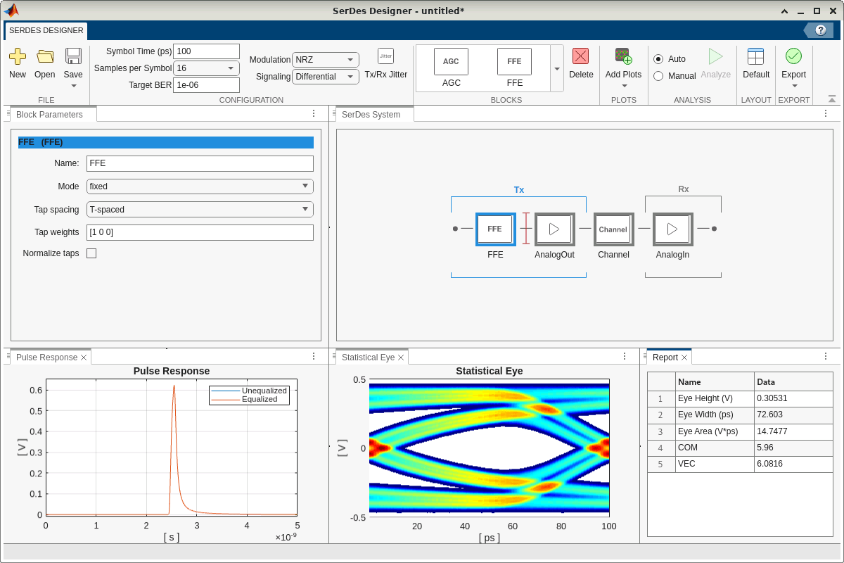
Add an FFE block to the left of the AnalogOut block of the transmitter side. Set Tap weights to [1 0 0] to configure this block as a 2-tap Tx FFE. Here the term 2-tap Tx FFE corresponds to three weights: one for the main tap associated with the current symbol being transmitted and two for the post-cursor taps that are used to correct mainly for frequency-dependent channel losses. These taps are part of the filter structure that is used to predistort the transmitted signal. Of course, given that the tap weights are currently set to [1 0 0], this FFE essentially acts as a no-op. Prior to manually tuning the FFE, the system remains unequalized, and the system performance metrics remain the same for now.

In addition, uncheck Normalize taps to disable automatic tap weight normalization. Instead, as shown in a later section, the optimization problem setup enforces the normalization condition—the sum of the absolute values of the tap weights is equal to unity—as a constraint.

Add 1-Tap Rx DFE

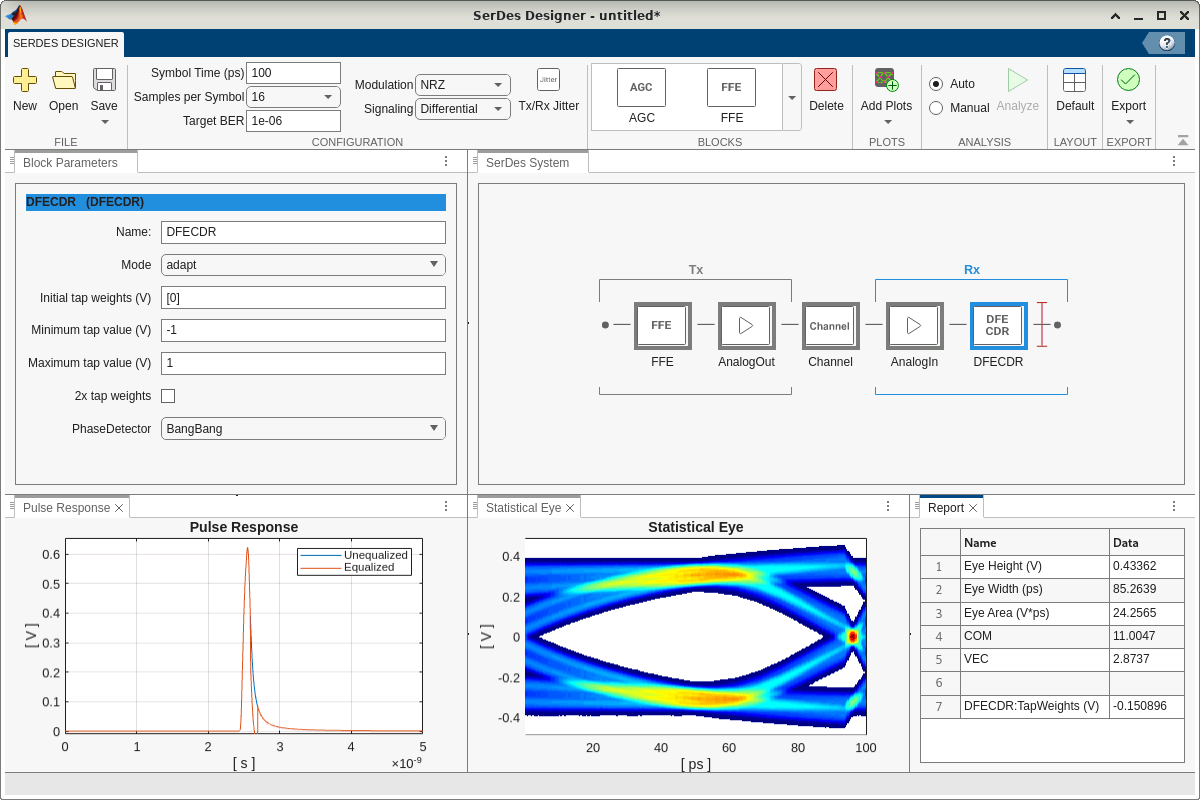
Add a DFECDR block to the right of the AnalogIn block of the receiver side. Set Initial tap weights (V) to [0] to configure this block as a 1-tap Rx DFE. Here the term 1-tap Rx DFE corresponds to one weight for the one feedback tap. This feedback mechanism is used to apply corrections to the current symbol based on previous symbol decisions to mitigate intersymbol interference (ISI). By default, Mode is set to adapt, which enables the block's built-in mechanism to automatically set the DFE tap weights to maximize eye height opening.

Evaluate Updated System Performance

Examine the Pulse Response, Statistical Eye, and Report above, all of which indicate improved system performance. Note that the improvement here is solely from the adaptive DFE, since the FFE is not yet tuned, as discussed earlier. Further improvement typically requires manual tuning of the FFE and DFE tap weights.

Configure Rx DFE to Disable Automatic Adaptation

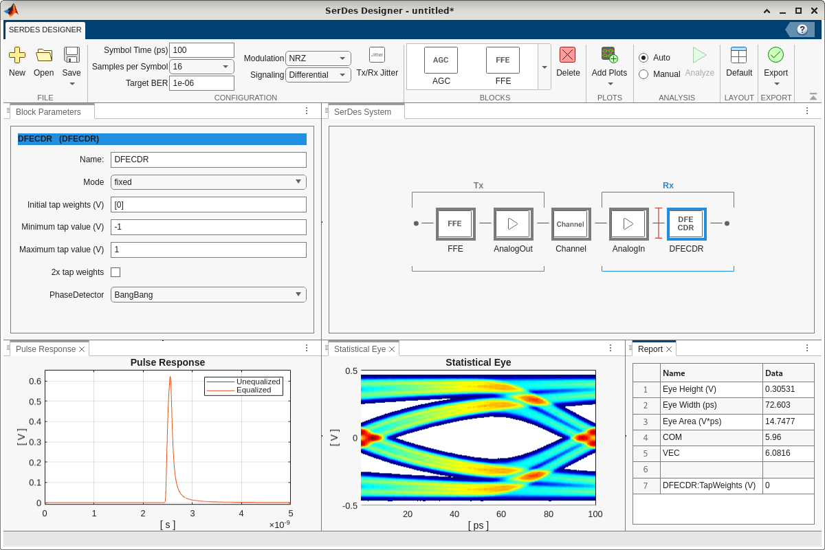
In the DFECDR block, set Mode to fixed to disable the block's built-in mechanism to automatically set the DFE tap value for best eye height opening. Instead, as shown in a later section, this example employs surrogate optimization separately to simultaneously optimize the DFE tap weight together with the FFE tap weights to maximize the eye area.

Export SerDes System from App to MATLAB Script

Navigate to the Export tab of the app toolstrip, and select Generate MATLAB code for SerDes System to automatically create a MATLAB script. This script contains the code to construct, tune, and analyze the SerDes system designed in the app. For reference and ease of comparison, this example includes the unmodified exported script in the helper file serdesExportedScript.m.

Create Optimization Objective Function from Exported Script

Formulate High Level Overview of Optimization Problem

The goal of the optimization task here is to select the weights for the Tx FFE and Rx DFE to maximize the statistical eye area. This optimization problem can be formulated as follows:

1. The objective is to maximize the eye area or, equivalently, to minimize the negative of the eye area.

2. There are four parameters to optimize: the three tap weights of the Tx FFE (${\mathit{x}}_1$ for the main tap, along with ${\mathit{x}}_2$ and ${\mathit{x}}_3$ for the two post-cursor taps) and the one tap weight of the Rx DFE (${\mathit{x}}_4$). Collectively, the optimization variable vector is $\mathit{x}=\left[\begin{array}{cccc}{\mathit{x}}_1& {\mathit{x}}_2& {\mathit{x}}_3& {\mathit{x}}_4\end{array}\right]$.

3. The search space for each of the tap weights is bounded as follows: $0.5\le {\mathit{x}}_1<1$ for the Tx FFE main tap, $-0.25\le {\mathit{x}}_2,{\mathit{x}}_3\le 0$ for each of the Tx FFE two post-cursor taps, and $-0.5\le {\mathit{x}}_4\le 0.5$ for the Rx DFE tap. These are reasonable, albeit slightly generous bounds on the tap values used in typical SerDes systems. These bounds also indirectly align with another constraint typically placed on the tap weights, namely that the absolute value of the main tap weight is greater than the absolute value of each of the non-main tap weights.

4. The Tx FFE tap weights are additionally constrained such that the sum of their absolute values is equal to unity. On the surface, this normalization condition appears to be a nonlinear equality constraint: $|{\mathit{x}}_1|+|{\mathit{x}}_2|+|{\mathit{x}}_3|=1$. However, in conjunction with the lower and upper bounds on the tap weights, this condition can be simplified and written as a linear equality constraint: ${\mathit{x}}_1-{\mathit{x}}_2-{\mathit{x}}_3=1$.

Modify Exported Script to Convert into Objective Function

Edit the generated MATLAB code as follows, starting with the exported script from the earlier section. For convenience, this example includes the final version of the objective function in the helper file serdesObjFcn.m. To see a summary of the changes, execute the following command.

visdiff("serdesExportedScript.m","serdesObjFcn.m")

First, configure the objective function argument syntax as follows:

• Accept as input the vector x of optimization parameters, specifically in the following order: the Tx FFE main tap and post-cursor tap weights, followed by the Rx DFE feedback tap weight.

• Also accept as input a figure handle fig and name-value pair Visualize used for visualization of the pulse response and eye diagram of the SerDes system for the provided tap weights. This aspect is optional and simply a convenience for diagnostic and visualization purposes. It is not required for the actual optimization task itself.

• Return as output the performance metric of interest: eye area. This is the quantity to optimize.

• Also return as output the SerdesSystem system object. This is not used by the optimizer, but it is provided as a convenience that is useful to later reconstruct the SerDes system using the optimized tap weights for further analysis and manual validation.

function [A,sys] = serdesObjFcn(x,fig,options)
% ---------------
% REQUIRED INPUTS
% ---------------
% x -- Weights for 2-tap Tx FFE and 1-tap Rx DFE:
%      [txMainTap,txPostCursorTap1,txPostCursorTap2,rxFeedbackTap1]
% 
% ---------------
% OPTIONAL INPUTS
% ---------------
% fig -- Figure handle in which to plot pulse response and eye diagram
%        (must be a matlab.ui.Figure if name-value pair Visualize=true)
% 
% ----------------
% NAME-VALUE PAIRS
% ----------------
% options.Visualize -- Logical scalar used to specify whether or not to
%                      plot pulse response and eye diagram (default: false)
% 
% -------
% OUTPUTS
% -------
% A -- Performance metric to optimize: eye area.
% sys -- SerDes system.

% Copyright 2024 The MathWorks, Inc.

arguments
    x (1,4) {mustBeNumeric}
    fig {mustBeScalarOrEmpty} = []
    options.Visualize (1,1) logical = false
end

if options.Visualize
    mustBeA(fig,"matlab.ui.Figure")
end

Next, in the section % Build cell array of Tx blocks, update the line that sets the TapWeights property to use the input optimization vector, x, instead of the fixed weights [1 0 0].

txBlocks{1}.TapWeights = x(1:3); % [1 0 0];

Similarly, in the section % Build cell array of Rx blocks, update the line that sets the TapWeights property to use x instead of the fixed weight 0.

rxBlocks{1}.TapWeights = x(4); % 0;

After the section % Build SerDes System, query the SerdesSystem system object to determine its eye area, which is used to calculate the objective function value.

% Return objective function output metrics: eye area
A = sys.Metrics.summary.eyeAreas;

Finally, at the end of the generated script, remove the plotting and exporting code. Instead, configure the objective function to optionally plot the pulse response and eye diagram while reusing the same figures and axis limits for all calls to the objective function across the optimization iterations. This can be used to visually track the evolution of the system pulse response and eye diagram as the optimizer searches through the parameter space. The last four lines shown below annotate the plots with the associated tap weights and corresponding eye area in each iteration. As mentioned earlier, this entire step is optional for diagnostics and convenience, and it not required for the optimization procedure.

% Visualize Pulse Response and Eye Diagram
if options.Visualize
    figure(fig)
    subplot(2,1,1)
    plotPulse(sys)
    xlim([2 3.5])
    ylim([-0.5 1])
    subplot(2,1,2)
    plotStatEye(sys)
    strTapWeights = mat2str([sys.TxModel.Blocks{1}.TapWeights, ...
        sys.RxModel.Blocks{1}.TapWeights],4);
    sgtitle("x = " + strTapWeights + newline + "Eye Area = " + A)
end

Use Surrogate Optimization to Determine Optimal Tx FFE and Rx DFE Tap Weights

Use the surrogateopt (Global Optimization Toolbox) function to optimize the tap weights to maximize the eye area while maintaining constraints (3) and (4) on the parameter values from the high level overview of the problem formulation.

Specify the lower and upper bounds constraints from (3). These satisfy the inequalities $\mathrm{lb3}\le \mathit{x}\le \mathrm{ub3}$.

lb3 = [0.5 -0.25 -0.25 -0.5];
ub3 = [1 0 0 0.5];

Specify the linear equality constraint from (4) in the form ${\mathit{A}}_{\mathrm{eq4}}\cdot \mathit{x}={\mathit{b}}_{\mathrm{eq4}}$.

• ${\mathit{A}}_{\mathrm{eq4}}$ is an ${\mathit{M}}_{\mathit{e}}$-by-${\mathit{n}}_{\mathrm{vars}}$ coefficient matrix, where ${\mathit{M}}_{\mathit{e}}=1$ is the number of constraint equalities, and ${\mathit{n}}_{\mathrm{vars}}=4$ is the number of optimization variables in $\mathit{x}$.

• ${\mathit{b}}_{\mathrm{eq4}}$ is a column vector of length 1 corresponding to the number of constraint equalities.

• The linear equality constraint from (4) can be written as ${\mathit{x}}_1-{\mathit{x}}_2-{\mathit{x}}_3+0\cdot {\mathit{x}}_4=1$. Note that there is only one equation and that the coefficient for ${\mathit{x}}_4$ is zero.

• Accordingly, ${\mathit{A}}_{\mathrm{eq4}}=\left[\begin{array}{cccc}1& -1& -1& 0\end{array}\right]$ and ${\mathit{b}}_{\mathrm{eq4}}=\left[\begin{array}{c}1\end{array}\right]$.

Aeq4 = [1 -1 -1 0];
beq4 = 1;

Configure the optimization search to begin with the tap weights [1 0 0 0]. This set of initial points correspond to the unequalized SerDes system, which is a reasonable and natural starting point.

x0 = [1 0 0 0];

Optionally, use the interactive check box control to visualize the pulse response and eye diagram for each iteration, but note that this will substantially slow down the cumulative execution time especially over large numbers of iterations.

animateVisualization = false;
if animateVisualization
    fig = figure;
else
    fig = [];
end

For the sake of reproducibility, reset the random number generator to its default state.

rng default

Run the surrogate optimization procedure. Note that the optimizer uses the negative of the output value returned by the serdesObjFcn helper function. This is to cast the optimization problem as a minimization problem. Also, note that there are no integer constraints and that there are no linear inequality constraints, and so these input arguments are set to []. Optionally, change the choice of the PlotFcn argument of the optimization options from optimplotfvalconstr to surrogateoptplot in order to see more detailed information about the solver's progress and optimization process.

tic
xOpt = surrogateopt(@(x)-serdesObjFcn(x,fig,Visualize=animateVisualization),lb3,ub3,[],[],[],Aeq4,beq4, ...
    optimoptions("surrogateopt",InitialPoints=x0,PlotFcn="optimplotfvalconstr"))

surrogateopt stopped because it exceeded the function evaluation limit set by 
'options.MaxFunctionEvaluations'.

xOpt = 1×4

    0.9192         0   -0.0808   -0.1515

toc

Elapsed time is 79.563496 seconds.

Verify and Validate Optimized Design

Use the serdesObjFcn helper function with the second output argument to retrieve the SerdesSystem system object with the FFE and DFE components configured to the optimal tap weights. Examine the pulse response, eye diagram, and other performance metrics for this optimized design.

figOpt = figure;
[~,sysOpt] = serdesObjFcn(xOpt,figOpt,Visualize=true)

sysOpt = 
  SerdesSystem with properties:

             TxModel: [1x1 Transmitter]
             RxModel: [1x1 Receiver]
                Name: []
          SymbolTime: 1.0000e-10
    SamplesPerSymbol: 16
          Modulation: 2
           Signaling: 'Differential'
           BERtarget: 1.0000e-06
         ChannelData: [1x1 ChannelData]
      JitterAndNoise: [1x1 JitterAndNoise]
                  dt: 6.2500e-12
     ImpulseResponse: [7065x1 double]
        ImpulseDelay: 2.4812e-09
                Wave: [1x1 struct]
                 Eye: [1x1 struct]
             Metrics: [1x1 struct]

sysOpt.Metrics.summary

ans = struct with fields:
              EH: 0.4664
          bestEH: 0.4800
              EW: 92.2757
             VEC: 1.4242
        eyeAreas: 27.9129
     COMestimate: 16.4070
    eyeLinearity: 1

Conclusion

In this example, you leveraged surrogate optimization to automatically determine optimal tap weights for FFE and DFE components in a SerDes system to maximize eye area, a quantitative performance metric. Specifically, you created an initial architectural design using the SerDes Designer app, exported this design to a MATLAB script, parameterized and modified the exported script to create an optimization objective function, used the surrogateopt function to find the optimal FFE and DFE tap weights, and then validated the optimized design by examining the pulse response, eye diagram, and other performance metrics. The verification results confirmed that this SerDes design optimization procedure is quick, successful, and automatable.

Related Examples

• Optimize Eye Height In SerDes System Model (Mixed-Signal Blockset)

More About

• What Is Surrogate Optimization? (Global Optimization Toolbox)