Design and Simulate Warehouse Pick-and-Place Application Using Mobile Manipulator in Simulink and Gazebo
This example shows how to set up an end-to-end, pick-and-place workflow for a mobile manipulator like the KINOVA® Gen3 on a Husky® mobile robot, in Simulink®.
Overview
This example simulates a mobile manipulator identifying and recycling objects into two bins using tools from these toolboxes:
Robotics System Toolbox™ — Models and simulates the manipulator.
Stateflow® — Schedules the high-level tasks in the example and step from task to task.
ROS Toolbox™ — Connects MATLAB® and Simulink to Gazebo®.
Computer Vision Toolbox™ and Deep Learning Toolbox™ — Perform object detection using a simulated camera in Gazebo.
This example builds on key concepts from the following related examples:
Plan and Execute Task- and Joint-Space Trajectories Using Kinova Gen3 Manipulator — Shows how to generate and simulate interpolated joint trajectories to move from an initial to a desired end-effector pose.
Pick-and-Place Workflow in Gazebo Using ROS — Shows how to setup an end-to-end pick and place workflow for a robotic manipulator like the KINOVA® Gen3 and simulate the robot in the Gazebo physics simulator.
Train YOLO v2 Network for Vehicle Detection (Computer Vision Toolbox) — Shows how to use a YOLO v2 object detector.
Get Started with Gazebo and Simulated TurtleBot (ROS Toolbox) — Shows how to set up the connection between MATLAB and Gazebo.
Robot Simulation and Control in Gazebo
This example uses Simulink to control two robots in Gazebo. Using ROS as the primary communication mechanism, enables you to use the allows the official Husky and KINOVA ROS packages for low-level motion control and sensing. This facilitates a straightforward transition from simulation to hardware, as the ROS commands stay the same.
The supplied Gazebo world also uses the Gazebo co-simulation plug-in, which enables direct MATLAB communication for tools such as querying the Gazebo world or directly setting the states of links in Gazebo.
Simulated sensors
Gazebo simulates these sensors:
RGB-D camera attached to the end-effector of the robot manipulator. The model uses this camera feed to detect objects to pick up.
2-D lidar sensor at the front of the mobile robot base. The model uses this laser feed to localize the robot in a precomputed map.
Pick-and-Place Workflow Using Simulink and Stateflow
In this example, the mobile manipulator operates in a simulated warehouse recycling facility, picking up recyclable objects from a central conveyor belt and transferring them to the corresponding recycling stations one by one.
The simulated recycling facility

The simulated mobile manipulator that is a Kinova Gen3 manipulator on a Husky mobile robot

Open the Simulink model to explore the pick-and-place components.
open_system('PickPlaceWorkflowSimulinkMobileArm.slx');

The Simulink model consists of these components:
MainTaskScheduler— This Stateflow chart schedules the tasks for the mobile manipulator to complete the pick-and-place job. It activates tasks for the robot manipulator or the mobile robot according to the required workflow.RobotManipulator— Implements tasks assigned to the robot manipulator by theMainTaskScheduler. This component consists of these main modules: the Robot Arm Scheduler, the Motion Planning subsystem and the Perception subsystem.MobileRobot— Implements tasks assigned to the mobile robot by the main scheduler. This component consists of these modules: the Mobile Robot Scheduler, the Path Planning subsystem and the Path Following subsystem.

1. Main Task Scheduler
The model implements the main workflow for the mobile manipulator by using a central Stateflow chart, which follows these steps:
The mobile manipulator navigates to the conveyor belt to pick up an object to recycle.
The RGB-D camera on the robot arm detects the poses and types of objects using deep learning.
The robot arm picks up the detected object.
The mobile manipulator navigates to the appropriate recycling bin for the detected object type (bottle or can) and places it.
The robot returns to the conveyor belt and repeats this workflow until no more objects are detected.

2. Robot Manipulator

A. Robot Arm Scheduler
The robot arm scheduler contains the Idle, MoveToHome, Detect, PickObject, and PlaceObject states. At any point in time, the robot arm is in one of these states, according to the task ordered by the Main Task Scheduler. To avoid conflict, if the robot arm or mobile robot is in a non-idle state, then the other must be in their idle state.

B. Motion Planning
The motion planning subsystem is an enabled subsystem that, once enabled by a signal from the robot arm scheduler, plans a trajectory and uses the ros-control package to send the command for tracking that trajectory to the joint trajectory controller running in ROS.
The robot arm scheduler sends a signal to enable this subsystem when the robot manipulator must move during the pick-and-place workflow. The subsystem remains enabled until the robot reaches the desired target pose. For more information in enabled subsystems, see Using Enabled Subsystems (Simulink).
C. Perception
The perception subsystem is a triggered subsystem that applies a pretrained deep learning model to the simulated end-effector camera feed from the robot to detect recyclable parts. The deep learning model takes a camera frame as input and outputs the 2-D location of the object (pixel position) and the type of recycling it requires (blue or green bin). The 2-D location in the image is mapped to the robot base frame using information about the camera properties (focal length and field of view), the input from the depth sensor, and the robot forward kinematics.
The robot manipulator task scheduler sends a signal to trigger this subsystem when the robot must detect the next object during the pick-and-place workflow. For more information on triggered subsystems, see Using Triggered Subsystems (Simulink).


3. Mobile robot
The Mobile Robot workflow consists of a Stateflow chart that governs the overall behavior of the mobile robot, a triggered subsystem that plans the path using a MATLAB function, and a the path following subsystem that uses control logic to follow the reference path.

Building Warehouse Space Map
In order to obtain a map of the workspace, you must first scan the environment. Mount a lidar sensor on the Husky to navigate around the environment and use the buildmap function to create an occupancy grid map. For more information, see Implement Simultaneous Localization And Mapping (SLAM) with Lidar Scans (Navigation Toolbox).
A. Mobile Robot Scheduler
The mobile robot scheduler contains the Idle, PlanPath, and FollowPath states. By default, the mobile robot is in the Idle state, meaning that the path planning and path following systems are inactive. The mobile robot scheduler receives task commands from the Main Task Scheduler. When the mobile robot scheduler receives a robot navigation task, it switches from the Idle state to the PlanPath state. The scheduler then continues to step, using feedback from the path planning and path following subsystems to advance through the stages, ultimately returning to the Idle state, which renders the task inactive and indicates to the Main Task Scheduler that it can move on with high-level tasks. The process then repeats given new inputs from the Main Task Scheduler.

B. Path Planning
During the PlanPath state, the mobile robot scheduler sets taskActive to true, which triggers the path planning subsystem. This subsystem contains a MATLAB function block that plans a path on the provided binary occupancy grid map using a plannerRRTStar object. The subsystem returns a set of path waypoints in SE(2), as well as a logical flag, isPath that indicates whether a path was successfully found.
Once the mobile robot scheduler receives a value of true for isPath, it advances to the FollowPath state.
C. Path following
In the FollowPath state, the mobile robot scheduler sets the requestFollowPath flag to true, which triggers the path following subsystem.

The subsystem has these main parts, listed in the order of execution:
Control Motion with Pure Pursuit — The Pure Pursuit block is the primary motion controller. Given the current pose of the robot and the upcoming waypoint, it assigns a velocity to move the robot to the waypoint.
Update Behaviors Given Distance to Goal — The
CheckDistancetoGoalandZero-VelocityatGoalsubsystems ensure that the robot stops when it has reached the goal. The model also uses the output from theCheck Distance to Goalsubsystem to verify task completion.Send Commands to Gazebo via ROS — The
BlankMessageandPublishblocks send the command linear and angular velocities from theZero-VelocityatGoalsubsystem to the appropriate velocity controller on the robot in Gazebo.
Together, these components drive the robot through the Gazebo world. Once the robot reaches the goal, the subsystem returns a value of true for atGoal, which indicates to the mobile robot scheduler that this state is complete.
Assign Variables for Use In Model
To run the Simulink model, you must assign some parameters related to the robot, default configurations, and target poses.
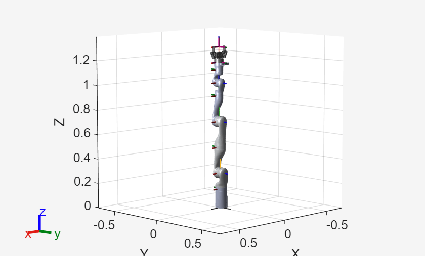
This simulation uses a KINOVA Gen3 manipulator attached to a Husky mobile robot. For the manipulator, a model of a KINOVA Gen3 with a gripper affixed is stored in a MAT file. Load the robot manipulator rigid body tree.
load("helperKINOVAGen3MobileArmPickPlace.mat");
show(robot);
axis auto
Initialize Pick and Place Application
Set the initial robot arm configuration and name of the end-effector body.
initialRobotJConfig = [1.583 0.086 -0.092 1.528 0.008 1.528 -0.08];
endEffectorFrame = "gripper";
Specify the home robot arm configuration and two poses for dropping objects of two different types. The first pose corresponds to the blue bin, for objects of type 1, and the second pose corresponds to the green bin, for objects of type 2.
homeArmPose = trvec2tform([0.0 -0.35 0.4])*axang2tform([0 0 1 -pi/2])*axang2tform([0 1 0 pi]);
detectionArmPose = trvec2tform([0.4 0.0 0.56])*axang2tform([0 0 1 -pi/2])*axang2tform([0 1 0 pi]);
placingArmPose = trvec2tform([0.6 0.0 0.57])*axang2tform([0 0 1 -pi/2])*axang2tform([0 1 0 pi/2])*axang2tform([1 0 0 -1.4]);
Specify the home mobile robot pose and two poses for dropping objects in the blue and green bins, depending on object type.
homeRobotPose = [7.95, 10.6, 0]; % x, y, theta
placingRobotPose2 =[13.16, 7.94, -0.92];
placingRobotPose1 = [15.15, 3.8, -1.752];
Set the step size for the simulation.
Ts = 0.1;
Start the Pick-and-Place Workflow
Start a ROS-based simulator for a KINOVA Gen3 robot and the configure MATLAB connection with the robot simulator. This example
Start Gazebo Simulation
This example uses a virtual machine (VM) containing ROS Melodic available for download here. This example does not support ROS Noetic as it relies on ROS packages which are only supported until ROS Melodic.
Start the Ubuntu® virtual machine desktop.
In the Ubuntu desktop, click the Mobile Manipulator World icon to start the Gazebo world built for this example, or run these commands:
source /opt/ros/melodic/setup.bash; source ~/catkin_ws/devel/setup.bash
export SVGA_VGPU10=0
export GAZEBO_PLUGIN_PATH=/home/user/src/GazeboPlugin/export:$GAZEBO_PLUGIN_PATH
roslaunch kortex_gazebo_depth mobilemanipulator.launch
Start ROS Master and Gazebo Interface Connection
Specify the IP address and port number of the ROS master in Gazebo so that MATLAB can communicate with the robot simulator. For this example, the ROS master in Gazebo is on 192.168.17.131:11311 and your host computer address is 192.168.17.1:61363. Replace these with the appropriate values corresponding to your ROS device setup. Start the ROS 1 network using rosinit.
rosIP = '192.168.17.131'; % IP address of ROS enabled machine
rosshutdown % shut down existing connection to ROS
Shutting down global node /matlab_global_node_93520 with NodeURI http://192.168.17.1:60235/ and MasterURI http://192.168.17.131:11311.
rosinit(rosIP,11311);
Initializing global node /matlab_global_node_18518 with NodeURI http://192.168.17.1:61756/ and MasterURI http://192.168.17.131:11311.
Initialize the Gazebo Interface using gzinit.
gzinit(rosIP);
Initialize Model
Set the initial arm pose in Gazebo using ROS.
configResp = helperSetCurrentRobotJConfig(initialRobotJConfig);
Unpause Gazebo physics.
physicsClient = rossvcclient("gazebo/unpause_physics");
physicsResp = call(physicsClient,"Timeout",3);
Load the precomputed map of the warehouse recycling facility.
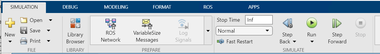
load("helperRecyclingWarehouseMap.mat");Start the workflow. Simulate the model by selecting Run on the Simulation tab.
 The model simulates until stopped.
Once both items have been moved, with the model still running, use the Gazebo MATLAB Interface to reset the positions of the red bottle and green can:
gzlink('set','Green Can','link','Position',[7.80007 11.2462 0.736121],'Orientation',[1 0 0 0]);
STATUS:  Succeed


MESSAGE:  Parameter set successfully.
gzlink('set','Red Bottle','link','Position',[7.932210479374374 11.287119941912177 0.783803767011424],'Orientation',[1 0 0 0]);
STATUS:  Succeed


MESSAGE:  Parameter set successfully.
You can also change the position values to try out the controller on different positions. The MATLAB interface enables you to control the Gazebo world directly from MATLAB, via commands by using functions such as gzlink and gzmodel.
To restart the model:
Close and re-run the script on the Ubuntu VM. Or if using the terminal and list of commands, simply close (Ctrl+C) and call the
roslaunchcommand again:
roslaunch kortex_gazebo_depth mobilemanipulator.launch
Run the setup commands starting from the Initialize Model section in MATLAB side and in Simulink, select Run.