Bias Mitigation in Credit Scoring by Reweighting
Bias mitigation is the process of removing bias from a data set or a model in order to make it fair. Bias mitigation usually follows a bias detection step, where a series of metrics are computed based on a data set or model predictions. Bias mitigation has three stages: pre-processing, in-processing, and post-processing. This example demonstrates a pre-processing method to mitigate bias in a credit scoring workflow. The example uses bias detection and bias mitigation functionality from the Statistics and Machine Learning Toolbox™. For a detailed example on bias detection, see the following example: Explore Fairness Metrics for Credit Scoring Model.
The bias mitigation method in this example is Reweighting which essentially reweights observations within a data set to guarantee fairness between different subgroups within a sensitive attribute. As a result of reweighting, the Statistical Parity Difference (SPD) of all subgroups goes to 0 and the Disparate Impact metric becomes 1. This example demonstrates how reweighting works in a credit scoring workflow.
Load Data
Load the CreditCardData data set and discretize the 'CustAge' predictor.
load CreditCardData.mat

AgeGroup = discretize(data.CustAge,[min(data.CustAge) 30 45 60 max(data.CustAge)], ...
    'categorical',{'Age < 30','30 <= Age < 45','45 <= Age < 60','Age >= 60'});

data = addvars(data,AgeGroup,'After','CustAge');
head(data)
    CustID    CustAge       AgeGroup       TmAtAddress    ResStatus     EmpStatus    CustIncome    TmWBank    OtherCC    AMBalance    UtilRate    status
    ______    _______    ______________    ___________    __________    _________    __________    _______    _______    _________    ________    ______

      1         53       45 <= Age < 60        62         Tenant        Unknown        50000         55         Yes       1055.9        0.22        0
      2         61       Age >= 60             22         Home Owner    Employed       52000         25         Yes       1161.6        0.24        0
      3         47       45 <= Age < 60        30         Tenant        Employed       37000         61         No        877.23        0.29        0
      4         50       45 <= Age < 60        75         Home Owner    Employed       53000         20         Yes       157.37        0.08        0
      5         68       Age >= 60             56         Home Owner    Employed       53000         14         Yes       561.84        0.11        0
      6         65       Age >= 60             13         Home Owner    Employed       48000         59         Yes       968.18        0.15        0
      7         34       30 <= Age < 45        32         Home Owner    Unknown        32000         26         Yes       717.82        0.02        1
      8         50       45 <= Age < 60        57         Other         Employed       51000         33         No        3041.2        0.13        0
Split the data set into training and testing data. Use the training data to fit the model and the testing data to predict from the model.
rng('default');
c = cvpartition(size(data,1),'HoldOut',0.3);
data_Train = data(c.training(),:);
data_Test = data(c.test(),:);
Compute Fairness Metrics at Predictor and Model Level
Compute the fairness metrics for the training data by creating a fairnessMetrics object and then generating a metrics report using report. Since you are only working with data and there is no fitted model, only two bias metrics are computed for StatisticalParityDifference and DisparateImpact. The two group metrics computed are GroupCount and GroupSizeRatio. The fairness metrics are computed for two sensitive attributes, Age ('AgeGroup') and Residential Status ('ResStatus').
trainingDataMetrics = fairnessMetrics(data_Train, 'status', 'SensitiveAttributeNames',{'AgeGroup', 'ResStatus'});
tdmReport = report(trainingDataMetrics)
tdmReport=7×4 table
    SensitiveAttributeNames        Groups        StatisticalParityDifference    DisparateImpact
    _______________________    ______________    ___________________________    _______________

           AgeGroup            Age < 30                   0.039827                   1.1357
           AgeGroup            30 <= Age < 45             0.096324                   1.3282
           AgeGroup            45 <= Age < 60                    0                        1
           AgeGroup            Age >= 60                  -0.19181                  0.34648
           ResStatus           Home Owner                        0                        1
           ResStatus           Tenant                      0.01689                   1.0529
           ResStatus           Other                      -0.02108                  0.93404
figure
tiledlayout(2,1)
nexttile
plot(trainingDataMetrics,'spd')
nexttile
plot(trainingDataMetrics,'di')

Looking at the DisparateImpact bias metric for both AgeGroup and ResStatus, you can see that there is a much larger variance in the AgeGroup predictor as compared to the ResStatus predictor. This suggests that users are treated more unfairly when it comes to their age as compared to their residential status. This example focuses on the AgeGroup predictor and attempts to reduce bias among its subgroups.
To begin, fit a credit scoring model and compute the model-level bias metrics. This provides a baseline for comparison.
Since CustAge and AgeGroup are essentially the same predictor and this is a sensitive attribute, you can exclude it from the model. Additionally, you can use 'status' as the response variable and 'CustID' as the ID variable.
PredictorVars = setdiff(data_Train.Properties.VariableNames, ...
    {'CustAge','AgeGroup','CustID','FairWeights','status'});
sc1 = creditscorecard(data_Train,'IDVar','CustID', ...
    'PredictorVars',PredictorVars,'ResponseVar','status');
sc1 = autobinning(sc1);
sc1 = fitmodel(sc1,'VariableSelection','fullmodel');
Generalized linear regression model:
    logit(status) ~ 1 + TmAtAddress + ResStatus + EmpStatus + CustIncome + TmWBank + OtherCC + AMBalance + UtilRate
    Distribution = Binomial

Estimated Coefficients:
                   Estimate       SE        tStat        pValue
                   ________    ________    ________    __________

    (Intercept)     0.73924    0.077237      9.5711     1.058e-21
    TmAtAddress      1.2577     0.99118      1.2689       0.20448
    ResStatus         1.755       1.295      1.3552       0.17535
    EmpStatus       0.88652     0.32232      2.7504     0.0059516
    CustIncome      0.95991     0.19645      4.8862    1.0281e-06
    TmWBank           1.132      0.3157      3.5856    0.00033637
    OtherCC         0.85227      2.1198     0.40204       0.68765
    AMBalance        1.0773     0.31969      3.3698    0.00075232
    UtilRate       -0.19784     0.59565    -0.33214       0.73978


840 observations, 831 error degrees of freedom
Dispersion: 1
Chi^2-statistic vs. constant model: 66.5, p-value = 2.44e-11
pointsinfo1 = displaypoints(sc1)
pointsinfo1=38×3 table
      Predictors              Bin            Points
    _______________    _________________    _________

    {'TmAtAddress'}    {'[-Inf,9)'     }     -0.17538
    {'TmAtAddress'}    {'[9,16)'       }      0.05434
    {'TmAtAddress'}    {'[16,23)'      }     0.096897
    {'TmAtAddress'}    {'[23,Inf]'     }      0.13984
    {'TmAtAddress'}    {'<missing>'    }          NaN
    {'ResStatus'  }    {'Tenant'       }    -0.017688
    {'ResStatus'  }    {'Home Owner'   }      0.11681
    {'ResStatus'  }    {'Other'        }      0.29011
    {'ResStatus'  }    {'<missing>'    }          NaN
    {'EmpStatus'  }    {'Unknown'      }    -0.097582
    {'EmpStatus'  }    {'Employed'     }      0.33162
    {'EmpStatus'  }    {'<missing>'    }          NaN
    {'CustIncome' }    {'[-Inf,30000)' }     -0.61962
    {'CustIncome' }    {'[30000,36000)'}     -0.10695
    {'CustIncome' }    {'[36000,40000)'}    0.0010845
    {'CustIncome' }    {'[40000,42000)'}     0.065532
      ⋮
pd1 = probdefault(sc1,data_Test);
Set the threshold value that controls the allocation of "goods" and "bads."
threshold = 0.35;
predictions1 = double(pd1>threshold);
0.35;
predictions1 = double(pd1>threshold);Create a fairnessMetrics object to compute fairness metrics at the model level and then generate a metrics report using report.
modelMetrics1 = fairnessMetrics(data_Test, 'status', 'Predictions', predictions1, 'SensitiveAttributeNames','AgeGroup');
mmReport1 = report(modelMetrics1)
mmReport1=4×7 table
ModelNames SensitiveAttributeNames Groups StatisticalParityDifference DisparateImpact EqualOpportunityDifference AverageAbsoluteOddsDifference
__________ _______________________ ______________ ___________________________ _______________ __________________________ _____________________________
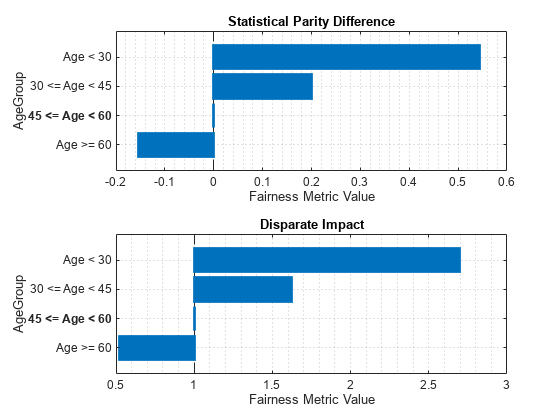
Model1 AgeGroup Age < 30 0.54312 2.6945 0.47391 0.5362
Model1 AgeGroup 30 <= Age < 45 0.19922 1.6216 0.35645 0.22138
Model1 AgeGroup 45 <= Age < 60 0 1 0 0
Model1 AgeGroup Age >= 60 -0.15385 0.52 -0.18323 0.16375
Measure accuracy of model using validatemodel.
validatemodel(sc1)
ans=4×2 table
            Measure              Value
    ________________________    _______

    {'Accuracy Ratio'      }    0.33751
    {'Area under ROC curve'}    0.66876
    {'KS statistic'        }    0.26418
    {'KS score'            }     1.0403
figure
tiledlayout(2,1)
nexttile
plot(modelMetrics1,'spd')
nexttile
plot(modelMetrics1,'di')
Reweight Data at Predictor and Model Level
Use fairnessWeights to reweight the training data to remove bias for the sensitive attribute 'AgeGroup'.
fairWeights = fairnessWeights(data_Train, 'AgeGroup', 'status');
data_Train.FairWeights = fairWeights;
head(data_Train)
    CustID    CustAge       AgeGroup       TmAtAddress    ResStatus     EmpStatus    CustIncome    TmWBank    OtherCC    AMBalance    UtilRate    status    FairWeights
    ______    _______    ______________    ___________    __________    _________    __________    _______    _______    _________    ________    ______    ___________

       1        53       45 <= Age < 60        62         Tenant        Unknown        50000         55         Yes       1055.9        0.22        0         0.95879
       2        61       Age >= 60             22         Home Owner    Employed       52000         25         Yes       1161.6        0.24        0         0.75407
       3        47       45 <= Age < 60        30         Tenant        Employed       37000         61         No        877.23        0.29        0         0.95879
       4        50       45 <= Age < 60        75         Home Owner    Employed       53000         20         Yes       157.37        0.08        0         0.95879
       7        34       30 <= Age < 45        32         Home Owner    Unknown        32000         26         Yes       717.82        0.02        1         0.82759
       8        50       45 <= Age < 60        57         Other         Employed       51000         33         No        3041.2        0.13        0         0.95879
       9        50       45 <= Age < 60        10         Tenant        Unknown        52000         25         Yes       115.56        0.02        1          1.0992
      10        49       45 <= Age < 60        30         Home Owner    Unknown        53000         23         Yes        718.5        0.17        1          1.0992
Use fairnessMetrics to compute fairness metrics for the training data after reweighting and use report to generate a fairness metrics report.
trainingDataMetrics_AfterReweighting = fairnessMetrics(data_Train, 'status', 'SensitiveAttributeNames','AgeGroup','Weights','FairWeights');
tdmrReport = report(trainingDataMetrics_AfterReweighting)
tdmrReport=4×4 table
    SensitiveAttributeNames        Groups        StatisticalParityDifference    DisparateImpact
    _______________________    ______________    ___________________________    _______________

           AgeGroup            Age < 30                  -2.9976e-15                   1
           AgeGroup            30 <= Age < 45            -5.5511e-16                   1
           AgeGroup            45 <= Age < 60                      0                   1
           AgeGroup            Age >= 60                 -2.9421e-15                   1
By applying the reweighting algorithm to the AgeGroup predictor, you can completely remove the disparate impact for AgeGroup. Then use this debiased data to fit a model to produce predictions with an overall reduced disparate impact at the model level.
Use creditscorecard to fit a new credit scoring model with the new fair weights and compute model-level bias metrics.
sc2 = creditscorecard(data_Train,'IDVar','CustID', ...
     'PredictorVars',PredictorVars,'WeightsVar','FairWeights','ResponseVar','status');
sc2 = autobinning(sc2);
sc2 = fitmodel(sc2,'VariableSelection','fullmodel');
Generalized linear regression model:
    logit(status) ~ 1 + TmAtAddress + ResStatus + EmpStatus + CustIncome + TmWBank + OtherCC + AMBalance + UtilRate
    Distribution = Binomial

Estimated Coefficients:
                   Estimate       SE        tStat        pValue
                   ________    ________    ________    __________

    (Intercept)     0.74055    0.076222      9.7158    2.5817e-22
    TmAtAddress      1.3416      0.9108       1.473       0.14075
    ResStatus        2.0467      1.7669      1.1584       0.24672
    EmpStatus       0.91879     0.32197      2.8536     0.0043222
    CustIncome      0.91038     0.33216      2.7407       0.00613
    TmWBank          1.1067     0.30826      3.5901     0.0003305
    OtherCC         0.42264      3.5078     0.12049        0.9041
    AMBalance        1.1347      0.3447      3.2919    0.00099504
    UtilRate       -0.39861     0.77284    -0.51577       0.60601


840 observations, 831 error degrees of freedom
Dispersion: 1
Chi^2-statistic vs. constant model: 46.6, p-value = 1.85e-07
pointsinfo2 = displaypoints(sc2)
pointsinfo2=34×3 table
      Predictors              Bin            Points
    _______________    _________________    ________

    {'TmAtAddress'}    {'[-Inf,9)'     }    -0.21328
    {'TmAtAddress'}    {'[9,23)'       }     0.07168
    {'TmAtAddress'}    {'[23,Inf]'     }     0.14763
    {'TmAtAddress'}    {'<missing>'    }         NaN
    {'ResStatus'  }    {'Tenant'       }    0.016048
    {'ResStatus'  }    {'Home Owner'   }    0.091092
    {'ResStatus'  }    {'Other'        }     0.28326
    {'ResStatus'  }    {'<missing>'    }         NaN
    {'EmpStatus'  }    {'Unknown'      }    -0.10352
    {'EmpStatus'  }    {'Employed'     }     0.33653
    {'EmpStatus'  }    {'<missing>'    }         NaN
    {'CustIncome' }    {'[-Inf,30000)' }    -0.37618
    {'CustIncome' }    {'[30000,40000)'}    0.047483
    {'CustIncome' }    {'[40000,42000)'}     0.10244
    {'CustIncome' }    {'[42000,47000)'}     0.14652
    {'CustIncome' }    {'[47000,Inf]'  }     0.40015
      ⋮
pd2 = probdefault(sc2,data_Test);
predictions2 = double(pd2>threshold);
Use fairnessMetrics to compute fairness metrics at the model level and report to generate a fairness metrics report.
modelMetrics2 = fairnessMetrics(data_Test, 'status', 'Predictions', predictions2, 'SensitiveAttributeNames','AgeGroup');
mmReport2 = report(modelMetrics2)
mmReport2=4×7 table
    ModelNames    SensitiveAttributeNames        Groups        StatisticalParityDifference    DisparateImpact    EqualOpportunityDifference    AverageAbsoluteOddsDifference
    __________    _______________________    ______________    ___________________________    _______________    __________________________    _____________________________

      Model1             AgeGroup            Age < 30                    0.39394                  2.1818                   0.37391                        0.39377
      Model1             AgeGroup            30 <= Age < 45             0.094298                  1.2829                   0.22947                        0.11509
      Model1             AgeGroup            45 <= Age < 60                    0                       1                         0                              0
      Model1             AgeGroup            Age >= 60                  -0.13333                     0.6                  -0.18323                         0.1511
Measure accuracy of model using validatemodel.
validatemodel(sc2)
ans=4×2 table
            Measure              Value
    ________________________    _______

    {'Accuracy Ratio'      }    0.27735
    {'Area under ROC curve'}    0.63868
    {'KS statistic'        }    0.22702
    {'KS score'            }    0.90741
figure
tiledlayout(2,1)
nexttile
plot(modelMetrics2,'spd')
nexttile
plot(modelMetrics2,'di')
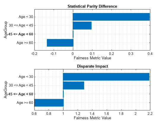
The process of reweighting removed all the bias from the training data. When you use the new data to fit a model, the overall bias in the model is reduced when compared to a model trained with biased data. As a consequence of this reduction in bias, there is a drop in model accuracy. You can choose to make tradeoff to improve fairness.
References
[1] Nielsen, Aileen. "Chapter 4. Fairness PreProcessing." Practical Fairness. O'Reilly Media, Inc., Dec. 2020.
[2] Mehrabi, Ninareh, et al. “A Survey on Bias and Fairness in Machine Learning.” ArXiv:1908.09635 [Cs], Sept. 2019. arXiv.org, https://arxiv.org/abs/1908.09635.
[3] Wachter, Sandra, et al. Bias Preservation in Machine Learning: The Legality of Fairness Metrics Under EU Non-Discrimination Law. SSRN Scholarly Paper, ID 3792772, Social Science Research Network, 15 Jan. 2021. papers.ssrn.com, https://papers.ssrn.com/sol3/papers.cfm?abstract_id=3792772.
See Also
creditscorecard | autobinning | fitmodel | displaypoints | probdefault