Train DQN Agent for Lane Keeping Assist Using Parallel Computing

This example uses:

This example shows how to train a deep Q-learning network (DQN) agent for lane keeping assist (LKA) in Simulink® using parallel training. For an example that shows how to train the agent without using parallel training, see Train DQN Agent for Lane Keeping Assist.

For more information on DQN agents, see Deep Q-Network (DQN) Agents. For an example that trains a DQN agent in MATLAB®, see Train DQN Agent to Balance Cart-Pole System.

DQN Parallel Training Overview

In a DQN agent, each worker generates new experiences from its copy of the agent and the environment. After every N steps, the worker sends experiences to the client agent (the agent associated with the MATLAB® process which starts the training). The client agent updates its parameters as follows.

For asynchronous training, the client agent calculates gradients and updates agent parameters from the received experiences, without waiting to receive experiences from all the workers. The client then sends the updated parameters back to the worker that provided the experiences. Then, the worker updates its copy of the agent and continues to generate experiences using its copy of the environment.
For synchronous training, the client agent waits to receive experiences from all of the workers and then calculates the gradients from all these experiences. The client updated the agent parameters, and sends the updated parameters to all the workers at the same time. Then, all workers use a single updated agent copy, together with their copy of the environment, to generate experiences.

Simulink Model for Ego Car

The reinforcement learning environment for this example is a simple bicycle model for the ego vehicle dynamics. The training goal is to keep the ego vehicle traveling along the centerline of the lanes by adjusting the front steering angle. This example uses the same vehicle model as Train DQN Agent for Lane Keeping Assist.

m = 1575;   % total vehicle mass (kg)
Iz = 2875;  % yaw moment of inertia (mNs^2)
lf = 1.2;   % longitudinal distance from center of gravity to front tires (m)
lr = 1.6;   % longitudinal distance from center of gravity to rear tires (m)
Cf = 19000; % cornering stiffness of front tires (N/rad)
Cr = 33000; % cornering stiffness of rear tires (N/rad)
Vx = 15;    % longitudinal velocity (m/s)

Define the sample time Ts and simulation duration T in seconds.

Ts = 0.1;
T = 15;

The output of the LKA system is the front steering angle of the ego car. To simulate the physical steering limits of the ego car, constrain the steering angle to the range [–0.5,0.5] rad.

u_min = -0.5;
u_max = 0.5;

The curvature of the road is defined by a constant 0.001 ( $m^{- 1}$ ). The initial value for the lateral deviation is 0.2 m and the initial value for the relative yaw angle is –0.1 rad.

rho = 0.001;
e1_initial = 0.2;
e2_initial = -0.1;

Open the model.

mdl = "rlLKAMdl";
open_system(mdl)
agentblk = mdl + "/RL Agent";

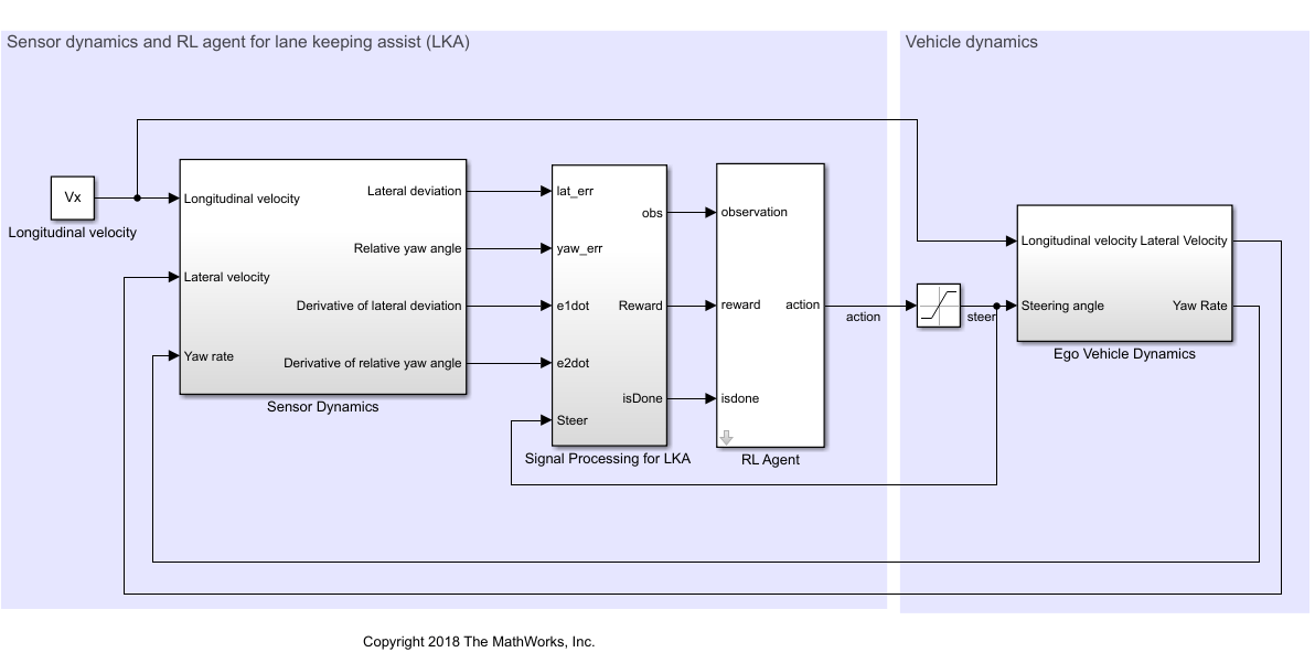
For this model:

The steering-angle action signal from the agent to the environment is from –15 degrees to 15 degrees.
The observations from the environment are the lateral deviation $e_{1}$ , relative yaw angle $e_{2}$ , their derivatives ${e_{}^{˙}}_{1}$ and ${e_{}^{˙}}_{2}$ , and their integrals $\int e_{1}$ and $\int e_{2}$ .
The simulation is terminated when the lateral deviation $| e_{1} | > 1 .$
The reward $r_{t}$ , provided at every time step $t$ , is

$r_{t} = - (10 e_{1}^{2} + 5 e_{2}^{2} + 2 u^{2} + 5 {e_{}^{˙}}_{1}^{2} + 5 {e_{}^{˙}}_{2}^{2})$

where $u$ is the control input from the previous time step $t - 1$ .

Create Environment Interface

Create a reinforcement learning environment interface for the ego vehicle.

Define the observation information.

obsInfo = rlNumericSpec([6 1], ...
    LowerLimit=-inf*ones(6,1), ...
    UpperLimit=inf*ones(6,1));

obsInfo.Name = "observations";
obsInfo.Description = "lateral deviation and relative yaw angle";

Define the action information.

actInfo = rlFiniteSetSpec((-15:15)*pi/180);
actInfo.Name = "steering";

Create the environment interface.

env = rlSimulinkEnv(mdl,agentblk,obsInfo,actInfo);

The interface has a discrete action space where the agent can apply one of 31 possible steering angles from –15 degrees to 15 degrees. The observation is the six-dimensional vector containing lateral deviation, relative yaw angle, as well as their derivatives and integrals with respect to time.

To define the initial condition for the lateral deviation and relative yaw angle, specify an environment reset function using an anonymous function handle. localResetFcn, which is defined at the end of this example, randomizes the initial lateral deviation and relative yaw angle.

env.ResetFcn = @(in)localResetFcn(in);

Create DQN Agent

DQN agents use a parametrized Q-value function approximator to estimate the value of the policy. Since DQN agents have a discrete action space, you have the option to create a vector (that is multi-output) Q-value function critic, which is generally more efficient than a comparable single-output critic.

A vector Q-value function takes only the observation as input and returns as output a single vector with as many elements as the number of possible actions. The value of each output element represents the expected discounted cumulative long-term reward when an agent starts from the state corresponding to the given observation and executes the action corresponding to the element number (and follows a given policy afterwards).

To model the parametrized Q-value function within the critic, use a neural network with one input (the six-dimensional observed state) and one output vector with 31 elements (evenly spaced steering angles from -15 to 15 degrees). Get the number of dimensions of the observation space and the number of elements of the discrete action space from the environment specifications.

nI = obsInfo.Dimension(1);      % number of inputs (6)
nL = 120;                       % number of neurons
nO = numel(actInfo.Elements);   % number of outputs (31)

Define the network as an array of layer objects.

dnn = [
    featureInputLayer(nI)
    fullyConnectedLayer(nL)
    reluLayer
    fullyConnectedLayer(nL)
    reluLayer
    fullyConnectedLayer(nO)
    ];

The critic network is initialized randomly. Ensure reproducibility by fixing the seed of the random generator.

rng(0)

Convert to a dlnetwork object and display the number of parameters.

dnn = dlnetwork(dnn);
summary(dnn)

   Initialized: true

   Number of learnables: 19.1k

   Inputs:
      1   'input'   6 features

View the network configuration.

plot(dnn)

Create the critic using dnn and the environment specifications. For more information on vector Q-value function approximators, see rlVectorQValueFunction.

critic = rlVectorQValueFunction(dnn,obsInfo,actInfo);

Specify training options for the critic using rlOptimizerOptions.

criticOptions = rlOptimizerOptions( ...
    LearnRate=1e-4, ...
    GradientThreshold=1, ...
    L2RegularizationFactor=1e-4);

Specify the DQN agent options using rlDQNAgentOptions, include the critic options object.

agentOpts = rlDQNAgentOptions(...
    SampleTime=Ts,...
    UseDoubleDQN=true,...
    CriticOptimizerOptions=criticOptions,...
    ExperienceBufferLength=1e6,...
    MiniBatchSize=256);

You can also set or modify the agent options using dot notation.

agentOpts.EpsilonGreedyExploration.EpsilonDecay = 1e-4;

Alternatively, you can create the agent first, and then access its option object and modify the options using dot notation.

Create the DQN agent using the specified critic and the agent options. For more information, see rlDQNAgent.

agent = rlDQNAgent(critic,agentOpts);

Training Options

To train the agent, first specify the training options. For this example, use the following options.

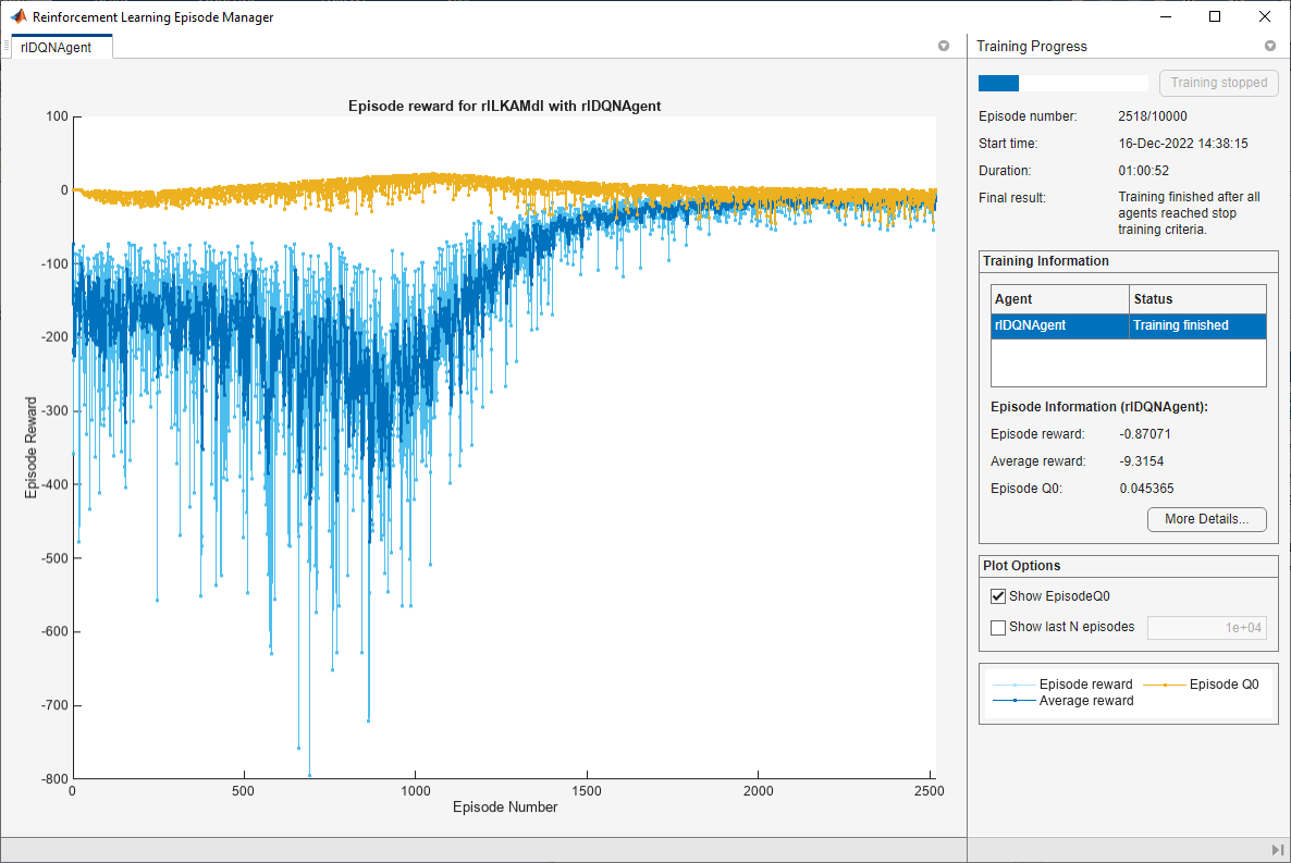
Run each training for at most 10000 episodes, with each episode lasting at most ceil(T/Ts) time steps.
Display the training progress in the Episode Manager dialog box only (set the Plots and Verbose options accordingly).
Stop training when the episode reward reaches -1.
Save a copy of the agent for each episode where the cumulative reward is greater than 100.

For more information, see rlTrainingOptions.

maxepisodes = 10000;
maxsteps = ceil(T/Ts);
trainOpts = rlTrainingOptions(...
    MaxEpisodes=maxepisodes, ...
    MaxStepsPerEpisode=maxsteps, ...
    Verbose=false,...
    Plots="training-progress",...
    StopTrainingCriteria="EpisodeReward",...
    StopTrainingValue= -1,...
    SaveAgentCriteria="EpisodeReward",...
    SaveAgentValue=100);

Parallel Training Options

To train the agent in parallel, specify the following training options.

Set the UseParallel option to true.
Train agent in parallel asynchronously by setting the ParallelizationOptions.Mode option to "async".

trainOpts.UseParallel = true;
trainOpts.ParallelizationOptions.Mode = "async";

For more information, see rlTrainingOptions.

Train Agent

Train the agent using the train function. Training the agent is a computationally intensive process that takes several minutes to complete. To save time while running this example, load a pretrained agent by setting doTraining to false. To train the agent yourself, set doTraining to true. Due to randomness of the parallel training, you can expect different training results from the plot below. The plot shows the result of training with four workers.

doTraining = false;

if doTraining
    % Train the agent.
    trainingStats = train(agent,env,trainOpts);
else
    % Load pretrained agent for the example.
    load("SimulinkLKADQNParallel.mat","agent")
end

Simulate the Agent

To validate the performance of the trained agent, uncomment the following two lines and simulate the agent within the environment. For more information on agent simulation, see rlSimulationOptions and sim.

% simOptions = rlSimulationOptions(MaxSteps=maxsteps);
% experience = sim(env,agent,simOptions);

To demonstrate the trained agent using deterministic initial conditions, simulate the model in Simulink.

e1_initial = -0.4;
e2_initial = 0.2;
sim(mdl)

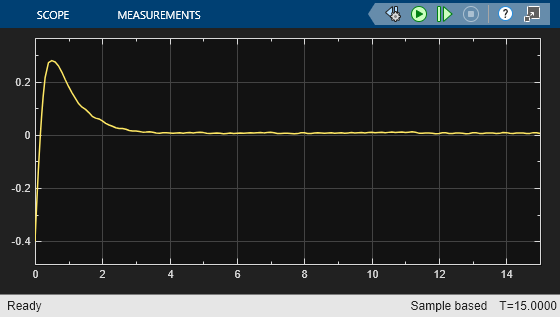
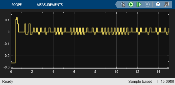
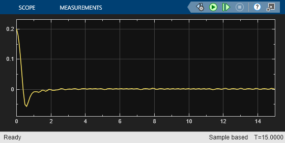
As shown below, the lateral error (middle plot) and relative yaw angle (bottom plot) are both driven to zero. The vehicle starts from off centerline (–0.4 m) and nonzero yaw angle error (0.2 rad). The LKA enables the ego car to travel along the centerline after 2.5 seconds. The steering angle (top plot) shows that the controller reaches steady state after 2 seconds.

Local Function

function in = localResetFcn(in)
% set initial lateral deviation and relative yaw angle to random values
in = setVariable(in,"e1_initial", 0.5*(-1+2*rand));
in = setVariable(in,"e2_initial", 0.1*(-1+2*rand));
end