Radar Design Part I: From Power Budget Analysis to Dynamic Scenario Simulation

Since R2024b

This example shows how to export a power-level Radar Designer session to an equivalent measurement-level model and simulate the radar and target in dynamic scenarios. In Radar Design Part II: From Radar Data to IQ Signal Synthesis, an equivalent waveform-level radar transceiver that simulates I/Q signals is created from the measurement-level model. The ability to export measurement-level radar models from the Radar Designer app allows you to efficiently test your radar hardware and software designs at the power-level (link budgets), measurement-level (detections), and waveform-level (IQ samples) and assess their performance on tasks like detection and tracking. This facilitates quicker design cycles and informed decision making.

Export a Data Generator from the Radar Designer

Launch the Radar Designer with preconfigured parameters for a fluctuating target moving radially away from the radar.

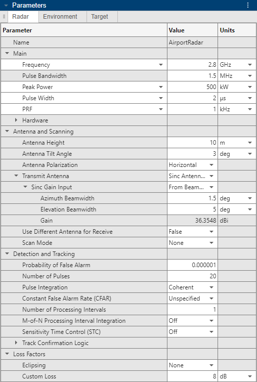
radarDesigner('AirportRadarFlucTarget.mat')

This example uses the default airport radar with the following changes:

• Peak Power of 500 kW (Radar Panel)

• Pulse Width of 2 microseconds (Radar Panel)

• Antenna Tilt Angle of 3 degrees (Radar Panel)

• No CFAR detection (set to "Unspecified" in the app) because we use a simpler thresholding algorithm in Radar Design Part II: From Radar Data to IQ Signal Synthesis of this example instead (Radar Panel)

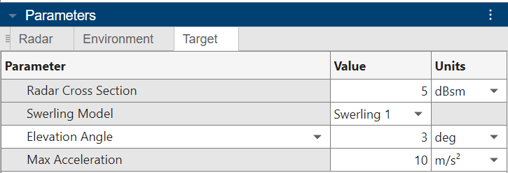
• Target RCS of 5 dBsm (Target Panel)

• Swerling I fluctuating target model (Target Panel)

• Target Elevation Angle of 3 degrees to match the antenna tilt angle (Target Panel)

You can adjust parameters in the radar and target panels on the left side of the app to create a radar that meets a given set of design requirements. Visualize key performance indicators in the metrics table at the bottom as well as in plots like SNR vs Range and Pd vs Range over the entire set of relevant ranges. More information on how to configure a radar in the app can be found in Radar Link Budget Analysis.

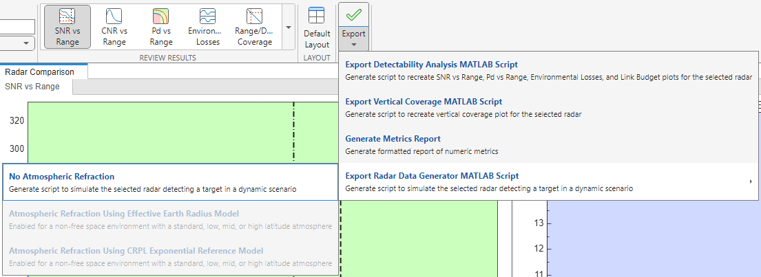
Next, export the Radar Designer configuration to a MATLAB script to create an equivalent measurement-level model of the radar and target. The script creates a radarDataGenerator System object™ (variable radarSensorModel) within a radarScenario (variable name scene) with a point target moving radially away from the radar at the elevation angle specified in the app. Navigate to the Export button on the toolstrip and select Export Radar Data Generator MATLAB Script, No Atmospheric Refraction. Running this script allows you to test your design in a dynamic radar scenario and populate the necessary radar and target properties in your workspace for more advanced applications and testing.

The rest of this example relies on loading previously exported scripts.

Running the MATLAB Script (Includes a Fluctuating Target)

The MATLAB script exported from the Radar Designer session configured in the previous section, models a point target moving radially away from the radar at an elevation of 3 degrees using radarDataGenerator. This elevation angle was chosen to match the antenna tilt angle of the radar so that the target stays in the center of the main radar beam. radarDataGenerator assumes a rectangular beam by default unless the ScanMode property is set to 'Custom' and the BeamShape property is set to 'Gaussian'.

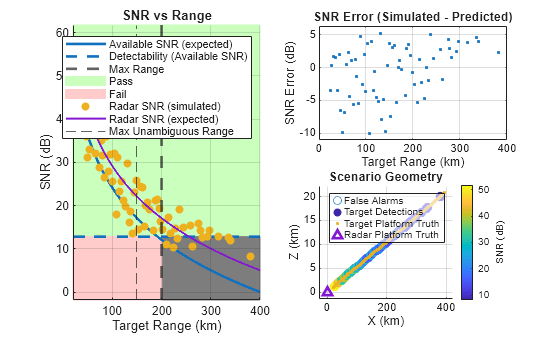
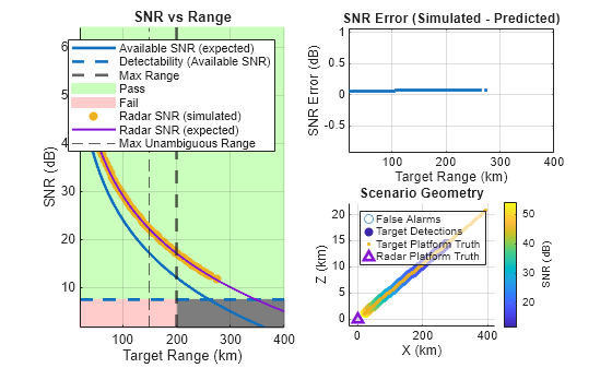
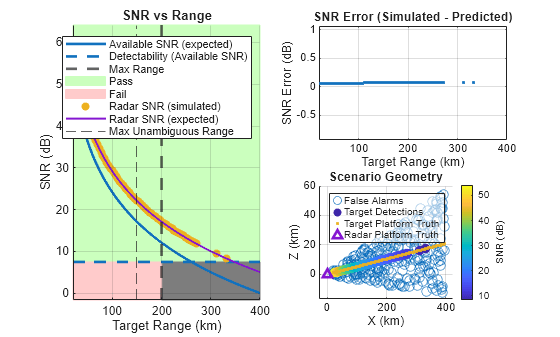
Running the exported script creates two figures. The first figure is an animated theaterPlot that shows the scenario geometry, radar field of view, and any detections. The second figure displays both a vertical cut of the scenario and an analysis of the simulation performance compared to the expected values from the Radar Designer app. In the second figure, there are three subplots.

• The leftmost plot shows SNR as a function of range for the radarDataGenerator detections and the SNRs predicted by Radar Designer for comparison. The table below summarizes these SNR curves. More information about the different SNRs and the processing gains and losses can also be found in Modeling Radar Detectability Factors. The curve labeled Radar SNR (simulated) should match closely with the curve labeled Radar SNR (expected) for a non-fluctuating target when all the radar properties defined in the Radar Designer are supported by radarDataGenerator. The target is fluctuating, leading to a distribution of reflected SNRs that match a Swerling I target model. More information concerning the different types of fluctuating targets can be found inIntroduction to Pulse Integration and Fluctuation Loss in Radar andSwerling Target Models.

SNR Curve	Description
Available SNR	Matches the plot seen in the Radar Designer app and represents the SNR at the receiver
Radar SNR (expected)	Available SNR plus any processing gains or losses
Radar SNR (simulated)	SNRs of the detections from the radarDataGenerator

• In the top right plot, the absolute difference between the Radar SNR (simulated) curve and the Radar SNR (expected) curve is shown. This error is less than 1 dB provided that the target is non-fluctuating and the radar properties selected in the app are supported by radarDataGenerator.

• In the bottom right plot, the scenario geometry is displayed along with the detections and false alarms. False alarms are only present if enabled in the radarDataGenerator, as explained in a following section.

rng('default') % Set the random number generator for reproducible results
run("Part_I_EXPORT_Swerling1.m") % Script exported from Radar Designer

customLossStaringRadar = radar.CustomLoss;
radarSensorClone = clone(radarSensorModel); % Save the radar from the original app configuration
targetClone = target; % Save the fluctuating target for later analysis

Non-Fluctuating Target

The above example includes a fluctuating target. To select a non-fluctuating target, you can either go to the Target panel in the app, change the Swerling Model to Swerling 0/5, and then re-export the script or you can simply scroll to where the Swerling case is set in the script and change it to 'Swerling0'. Note that changing a non-fluctuating target to a fluctuating target in the script can lead to errors because the fluctuation loss is not included in the detectabilityComponents() function unless a fluctuating target is exported from the app.

In the script, locate the instantiation of the target structure and change

target.SwerlingCase = 'Swerling1';

to

target.SwerlingCase = 'Swerling0';

and then

run("Part_I_EXPORT_Swerling0.m")

As shown above, for the non-fluctuating target case, the absolute SNR error remains below 0.1 dB for all detections.

Add Position Estimation Noise

Noise in the position estimation of the detections can also be modeled by radarDataGenerator. This can be seen in the scenario geometry plot. Note that the detections are no longer at a constant elevation angle and noise is only applied to the position estimation of the detections and not to the SNR of the detections. For a non-fluctuating target (shown below), a plot of the SNR vs ground truth range yields a negligible error.

In the script, locate the instantiation of the radarDataGenerator and change

'HasNoise', false, ... % Target position noise

to

'HasNoise', true, ... % Target position noise

and then

run('Part_I_EXPORT_Swerling0_Noise.m')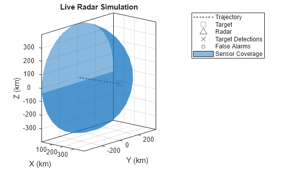

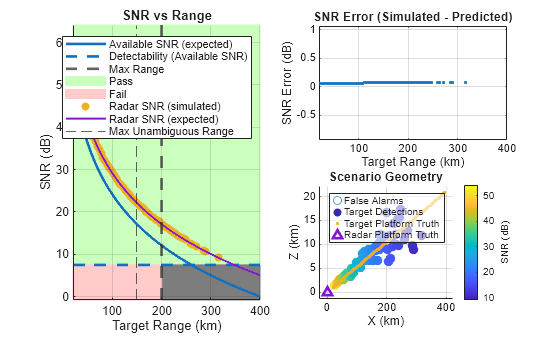
False Alarms

The false alarm rate is set in the Radar Designer app within the Radar panel. Enabling this option within the radarDataGenerator generates false alarms within the field of view of the radar. To see the impact of false alarms for the default value of 1e-6, locate the instantiation of the radarDataGenerator and change

'HasFalseAlarms', false, ...

'FieldOfView', [180,180], ... % (deg) Change to the effective beamwidths to limit detections to the half-power beamwidths

to

'HasFalseAlarms', true, ...

'FieldOfView', [30,10], ... % (deg) Change to the effective beamwidths to limit detections to the half-power beamwidths

and then

run('Part_I_EXPORT_Swerling0_FalseAlarm.m')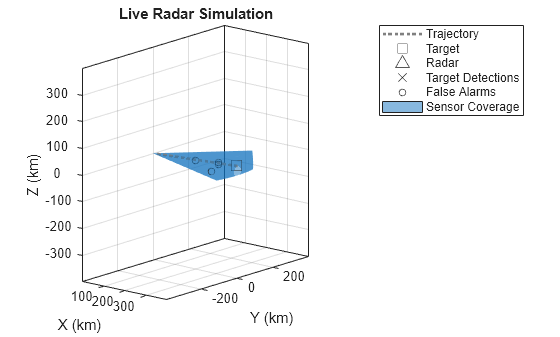

Scanning Radar

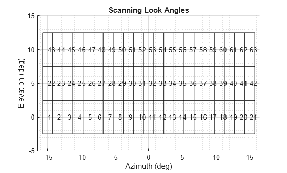
Both mechanical and electronic scanning can be modeled in the Radar Designer app. Mechanical scanning covers the field of interest using an S-like pattern while Electronic scanning scans from left to right and then jumps back to the left limit and then begins its next horizontal scan, as shown in Simulate a Scanning Radar. To see the configurable scanning options, set the scan mode to electronic or mechanical in the Radar panel. Below is one possible scanning configuration.

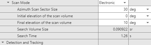
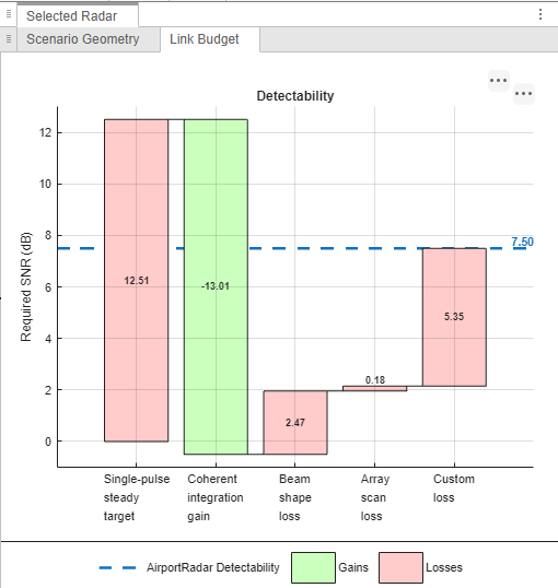
The search time in the app is computed by multiplying the dwell time (number of pulses within one processing interval divided by the PRF) by the number of look angles necessary to cover the 2D scan limits given the beamwidth in each dimension. In the configuration depicted immediately above, there are 63 look angles, each taking 1 ms, totaling 1.26 s for the search time. These 63 look angles can be visualized in the lower-most plot. Also, note that there are less detections in this scenario because the target is not in the scanning field of view for most look angles. The combined beam shape and array scan loss is 2.65 dB. To keep the SNR values consistent with the previous demonstrations (and for the rest of this example), add a gain to the radar that compensates for the new losses. A convenient way to do this is to reduce the custom loss in the Radar panel by the combined beam shape and array scan loss. As a result, the custom loss should be set to 5.35 dB which is the original custom loss of 8 dB minus the beam shape and array scan loss of 2.65 dB. Export the updated design and run the script.

run('Part_I_EXPORT_Swerling0_Scanning.m')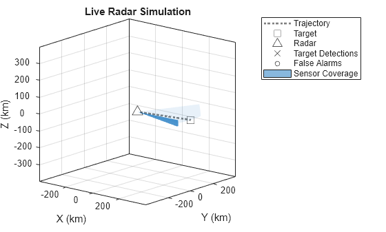

scanningRadarSensorClone = radarSensorModel; % Save for later use

Test the Probability of Detection

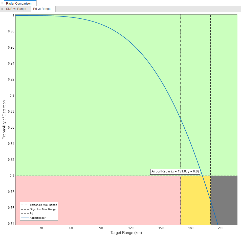
Probability of detection is also calculated by Radar Designer and modeled by radarDataGenerator. To verify the probability of detection values, first, open the Radar Designer app again and navigate to the Pd vs Range button in the Review Results area of the toolstrip. Then, pick a point on this curve and set the position of the point target to remain at that range from the radar. For this example, set the range to 191.77 km and use the Pd vs Range plot to find the corresponding probability of detection, which is approximately 80%.

Next, model the probability of detection with radarDataGenerator by taking a Monte-Carlo approach. Simulate the static target located at 191.77 km for 1000 iterations and divide the number of detections by the total number of transmissions. (The colors in the app disappear when there are multiple radars.) Run the following commands in your workspace.

rng('default') % Set the random number generator for reproducible results
target = targetClone; % Fluctuating target from the original export from the app
radarSensorModel = radarSensorClone; % Original radar configuration from the app
reset(radarSensorModel)
updateRate = .1; % (Hz)
scene = radarScenario('UpdateRate',updateRate);

% Place radar on a stationary platform
radarPos = [0,0,radar.Height]; % East-North-Up Cartesian Coordinates
radarOrientation = [0 0 0];  % (deg) Yaw, Pitch, Roll
radarPlat = platform(scene,'Position',radarPos,'Sensors',radarSensorModel,'Orientation',radarOrientation);

% Place a static target within the detectable range of the radar
targetPlat = platform(scene,'Position',191.77e3*[cosd(target.ElevationAngle) 0 sind(target.ElevationAngle)], ...
    'Signatures',{rcsSignature('Pattern',ones(2,2)*pow2db(target.RCS), ...
    'FluctuationModel',target.SwerlingCase)});

% Run Monte-Carlo Experiment to Test Detectability
T = 10000; % (s) Time of arrival of target at final position
n=1;
simDet = zeros(ceil(T*updateRate+1),1);
while n <= numel(simDet)
    dets = detect(scene);
    if ~isempty(dets)
        simDet(n) = 1;
    end
    n = n+1;
end
mean(simDet)

ans = 
0.8122

Test the Measurement-Level Radar in a New Scenario

Now that the radarDataGenerator is configured, you can easily test your new design in different and more complicated scenarios. In this example, create four static targets at different locations.

% Create Theater Plot and Plotters
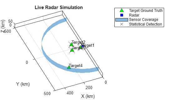
[scene,tp] = helperConstructScene(radarSensorModel, radar, true);

Simulate the Staring Radar in a New Scenario

The simulation yields a detection for the three closest targets and produces a missed detection for the farthest target.

rng('default') % Set the random number generator for reproducible results
reset(radarSensorModel) % Allows you to rerun the radar

detBuffer = {};
while advance(scene)
    [dets, config] = detect(scene);

    detBuffer = [detBuffer;dets]; %#ok<AGROW>

    % Is full scan complete?
    if config.IsScanDone
        break % yes
    end
end
statStaringDets = detBuffer; % Save results for final comparison
detPos = zeros(numel(detBuffer),3);
for m = 1:numel(detBuffer)
    detPos(m,:) = detBuffer{m}.Measurement(1:3).';
end
% Plot the detections on the theater plot
statDetPlotter = detectionPlotter(tp,'DisplayName','Statistical Detection',...
    'Marker','x','MarkerSize',20);
plotDetection(statDetPlotter,detPos)

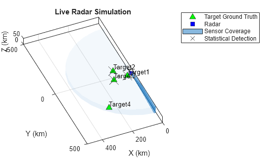
Simulate the Scanning Radar in a New Scenario

Just like the scenario can be modified, the radar system itself can be modified once the radar sensor is in the exported script. This allows you to enable features that are not supported by the Radar Designer app or by the automated export process. In this example, we change the scan limits to accommodate the four new targets. For the purpose of speeding up this example, we will also extend the field of view in the elevation axis. Note, extending the beamwidth in the Radar Designer would automatically result in a lower antenna gain (which is ignored by changing it in this manner).

rng('default') % Set the random number generator for reproducible results
release(scanningRadarSensorClone) % Allows us to modify the radar

scanningRadarSensorClone.FieldOfView(2) = 60; % elevation, deg
scanningRadarSensorClone.ElectronicElevationLimits = [0 45];      % deg
scanningRadarSensorClone.ElectronicAzimuthLimits = [-90 90];      % deg

[scene,tp,FOVPlotter] = helperConstructScene(scanningRadarSensorClone, radar, true);

detBuffer = {};
% Run Simulation
while advance(scene)
    plotCoverage(FOVPlotter,coverageConfig(scanningRadarSensorClone))
    [dets, config] = detect(scene);

    detBuffer = [detBuffer;dets]; %#ok<AGROW>

    % Is full scan complete?
    if config.IsScanDone
        break % yes
    end
    pause(.001)
end
statScanningDets = detBuffer; % Save results for final comparison
% Plot the detections on the theater plot
detPos = zeros(numel(detBuffer),3);
for m = 1:numel(detBuffer)
    detPos(m,:) = detBuffer{m}.Measurement(1:3).';
end
statDetPlotter = detectionPlotter(tp,'DisplayName','Statistical Detection',...
    'Marker','x','MarkerSize',20);
plotDetection(statDetPlotter,detPos)

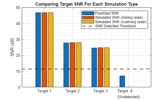
Compare Results From Radar Designer and radarDataGenerator

Here we compare the SNRs of the two radar simulators:

1. Radar Designer App

2. Measurement-Level Staring Radar

3. Measurement-Level Scanning Radar

rgs = helperGetTargetRanges(scene); % (m) Ranges of targets

% Radar Designer App
radarSNRExpected = availableSNR + pow2db(radar.NumCoherentPulses) - customLossStaringRadar; % expected SNR (with processing gain) for non-fluctuating target
appSNR = interp1(target.ranges,radarSNRExpected,rgs);

% Staring Radar
statStaringSNRs = helperSortSNRs(statStaringDets);
statStaringSNRs = [statStaringSNRs; NaN];

% Scanning Radar
statScanningSNRs = helperSortSNRs(statScanningDets);
statScanningSNRs = [statScanningSNRs; NaN];

figure
bar(["Target 1","Target 2","Target 3","Target 4\newline(Undetected)"],[appSNR statStaringSNRs statScanningSNRs]')
yline(npwgnthresh(radar.Pfa),'LineWidth',2,'LineStyle','--')
ylabel('SNR (dB)')
title('Comparing Target SNR For Each Simulation Type')
grid
grid minor
legend('Predicted SNR', 'Simulated SNR (staring radar)','Simulated SNR (scanning radar)','SNR Detection Threshold')

% Save results for Part II results comparison 
data.results = [appSNR statStaringSNRs statScanningSNRs];
data.labels = ["Power-Level Prediction", "Measurement-Level Staring Radar","Measurement-Level Scanning Radar"];
save('AppAndStatResults.mat','-struct','data');

Summary

This example demonstrated how to go from the Radar Designer app to a measurement-level model of a radar. Both the measurement-level SNR and probability of detection are consistent with the power-level predictions from the Radar Designer app. You saw how straightforward it was to change both the radar sensor and the radar scenario by modifying the generated script or by running entirely new code after the workspace has been set.

Helper Functions

% Define targets in the scenario (same as in Part II of this example series)
function [tgt1, tgt2, tgt3, tgt4] = helperCreateTargets(scene)
    tgt1 = platform(scene, ...
        'ClassID',1, ... % set to 1 for targets
        'Position',[30e3 20e3 5e3], ...
        'Signatures',{rcsSignature(Pattern=5)}); % (dBsm)
    tgt2 = platform(scene, ...
        'ClassID',1, ...
        'Position',[95e3 -50e3 10e3], ...
        'Signatures',{rcsSignature(Pattern=5)}); % (dBsm)
    tgt3 = platform(scene, ...
        'ClassID',1, ...
        'Position',[125e3 30e3 12e3], ...
        'Signatures',{rcsSignature(Pattern=5)}); % (dBsm)
    tgt4 = platform(scene, ...
        'ClassID',1, ...
        'Position',[250e3 250e3 5e3], ...
        'Signatures',{rcsSignature(Pattern=5)}); % (dBsm)
end

% Construct radar scenario and dynamic plot
function [scene, tp, FOVPlotter] = helperConstructScene(radarSensorModel, radar, plotFlag)    
    
    scene = radarScenario('UpdateRate',0); % UpdateRate of 0 updates when new measurement is available
    
    % Define Targets
    [tgt1, tgt2, tgt3, tgt4] = helperCreateTargets(scene);
    
    % Define Radar Platform
    radarPos = [0,0,radar.Height]; % East-North-Up Cartesian Coordinates
    radarOrientation = [0 0 0];  % (deg) Yaw, Pitch, Roll
    % ClassID of the radar is 2 while the targets are set to 1
    radarPlat = platform(scene,'ClassID',2,'Position',radarPos,'Sensors',radarSensorModel,'Orientation',radarOrientation);
    
    tp = false;
    if plotFlag
        tp = theaterPlot('XLimits',[0 500e3],'YLimits',[-500e3 500e3],'ZLimits',[0,50e3],...
            'AxesUnits',["km","km","km"]);
        legend('Location','northeast','BackgroundAlpha',.6)
        title('Live Radar Simulation')
        view(157,41);grid on;
    
        % Plot Target Ground Truths
        gtplot = platformPlotter(tp,'DisplayName','Target Ground Truth',...
            'Marker','^','MarkerSize',8,'MarkerFaceColor','g');
        plotPlatform(gtplot,[tgt1.Position;tgt2.Position;tgt3.Position;tgt4.Position],{'Target1','Target2','Target3','Target4'});
    
        % Plot Radar
        radarplot = platformPlotter(tp,'DisplayName','Radar',...
            'Marker','s','MarkerSize',8,'MarkerFaceColor','b');
        plotPlatform(radarplot, radarPlat.Position,...
                radarPlat.Dimensions,quaternion(radarPlat.Orientation,'rotvecd'))
        
        % Plot Radar Field of View / Coverage
        FOVPlotter = coveragePlotter(tp,'DisplayName','Sensor Coverage');
        plotCoverage(FOVPlotter,coverageConfig(radarPlat.Sensors{1}))
    end
end

% Find the target platforms' ranges relative to radar
function rgs = helperGetTargetRanges(scene)
    plats = scene.Platforms;
    radarPlatIdx = cell2mat(cellfun(@(x) x.ClassID==2,plats,'UniformOutput',false));

    targetPosesVector = targetPoses(plats{radarPlatIdx}); % Relative to radar platform
    rgs = zeros(numel(plats)-1,1);

    for ii = 1:numel(targetPosesVector)
        rgs(ii) = norm(targetPosesVector(ii).Position);
    end
end

% Sort SNRs according to target indexes
function SNRVector = helperSortSNRs(dets)
    targetIdx = cellfun(@(x) x.ObjectAttributes{1,1}.TargetIndex, dets, 'UniformOutput', 1);
    [~,sortIdx] = sort(targetIdx,'ascend');
    SNRVector = cellfun(@(x) x.ObjectAttributes{1,1}.SNR, dets, 'UniformOutput', 1);
    SNRVector = SNRVector(sortIdx);
end