Modeling Radar Detectability Factors

Since R2021a

This example shows how to model antenna, transmitter, and receiver gains and losses for a detailed radar range equation analysis. We start by computing the available signal-to-noise ratio (SNR) at the radar receiver using the SNR form of the radar equation. Next, we define the detectability factor as a threshold SNR required to make a detection with specified probabilities of detection, $$P_d$$, and false alarm, $$P_{fa}$$. We then estimate the maximum range of the system as the range at which the available SNR is equal to the detectability factor, that is the maximum range at which the detection with the specified $$P_d$$ and $$P_{fa}$$ is still possible. The example further explores the impact of losses introduced by different components of the radar system on the estimated maximum range. We first consider the effects of the sensitivity time control (STC) and eclipsing on the available SNR. Scanning and signal processing losses that require an increase in the radar detectability factor are considered next. The example concludes by computing the resulting $$P_d$$ at the detector output to show the impact of the losses on the detection performance of the radar system.

Available SNR

The radar equation combines the main parameters of a radar system and allows a radar engineer to compute a maximum detection range, a required peak transmit power, or a maximum available SNR for a radar system. The radar equation is typically a family of relatively simple formulas each corresponding to one of these three key performance characteristics. A common form of the radar equation for computing the maximum available SNR at a range $$R$$ is:

$$SNR=\frac{P_t\tau G_t{G}_r{\lambda }^2\sigma }{(4\pi {)}^{3}k{T}_s{R}^{4}L}$$

where

$$P_t$$ is the peak transmit power

$$\tau$$ is the transmitted pulse width

$$G_t$$ is the transmit antenna gain

$$G_r$$ is the receive antenna gain

$$\lambda$$ is the radar wavelength

$$\sigma$$ is the radar target cross section (RCS)

$$k$$ is Boltzmann's constant

$$T_s$$ is the system noise temperature

$$L$$ is the general loss factor that combines losses along the transmitter-target-receiver path that reduce the received signal energy.

On the right-hand side all parameters except the target range and RCS are under control of the radar designer. This equation states that for a target of a given size located at a range $$R$$, the SNR available at the receiver can be increased by transmitting more power, increasing the antenna size, using lower frequency, or having a more sensitive receiver.

Consider an S-band airport surveillance radar operating at the frequency of 3 GHz. The peak transmit power is 0.2 MW, the transmit and receive antenna gain is 34 dB, the pulse duration is 11 $\mu$s, and the noise figure is 4.1 dB. Assume the radar is required to detect a target with 1 m$${}^2$$ RCS at the maximum range $$R_m$$ of 100 km.

lambda = freq2wavelen(3e9);         % Wavelength (m)
Pt = 0.2e6;                         % Peak power (W)
tau = 1.1e-5;                       % Pulse width (s)
G = 34;                             % Transmit and receive antenna gain (dB)
Ts = systemp(4.1);                  % System temperature (K) 
rcs = 1;                            % Target radar cross section (m^2)
Rm = 100e3;                         % Required maximum range (m)

To start, assume no losses, that is $$L$$ = 0 dB. We use the radar equation to compute the available SNR at the receiver as a function of target range.

L = 0;                              % Combined transmission line and propagation losses (dB)
R = (1:40:130e3).';                 % Range samples (m)
SNR = radareqsnr(lambda,R,Pt,tau,'Gain',G,'Ts',Ts,'RCS',rcs,'Loss',L);

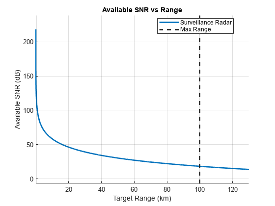
Calculate the available SNR at the required maximum range of 100 km.

SNRatRm = SNR(find(R>=Rm,1))

SNRatRm = 
18.3169

Plot the maximum range requirement together with the computed available SNR.

radarmetricplot(R*1e-3,SNR,'MetricName','Available SNR','MaxRangeRequirement',Rm*1e-3,...
    'RangeUnit','km','MetricUnit','dB','RadarName',{'Surveillance Radar'});
legend('Location','best');

Required SNR

Is the computed available SNR high enough to make a detection? Since the signal processed by a radar receiver is a combination of the transmitted waveform and the random noise, the answer to this question depends on the desired probability of detection $$P_d$$ and the maximum acceptable probability of false alarm $$P_{fa}$$. These probabilities define the required SNR, also known as the detectability factor (or detectability). The detectability factor is the minimum SNR required to declare a detection with the specified probabilities of detection and false alarm. It also depends on the RCS fluctuation and the type of the detector. Compute the detectability factor for a single pulse received from a steady (Swerling 0) target by a square-law detector assuming $$P_d$$ = 0.9 and $$P_{fa}$$ = 1e-6.

Pd = 0.9;
Pfa = 1e-6;
D0 = detectability(Pd,Pfa,1,'Swerling0')

D0 = 
13.1217

Calculate the detectability factor for a Swerling 1 fluctuating target, which is a more accurate model for real-world targets. For the Swerling 1 target the single-pulse detectability factor is significantly higher.

D1 = detectability(Pd,Pfa,1,'Swerling1')

D1 = 
21.1436

The resultant required SNR is higher than the available SNR, which means that a Swerling 1 target will not be detected with a single pulse. A common way to lower the detectability factor is to perform pulse integration. Calculate the detectability factor for $$N$$ = 10 noncoherently integrated pulses.

N = 10;
DN = detectability(Pd,Pfa,N,'Swerling1')

DN = 
13.5033

This is lower than the available SNR. Thus, after a non-coherent integration of 10 pulses the radar system will be able to detect a 1 m$${}^2$$ target at the required maximum range of 100 km with the probability of detection 0.9 and a false alarm of 1e-6.

The detectability factor computed for a Swerling 1 target and $$N$$ pulses combines the effects of the integration gain and the fluctuation loss. The integration gain is a difference between the SNR required to detect a steady target using a single pulse and the SNR required to detect a steady target using $$N$$ pulses.

Gi = detectability(Pd,Pfa,1,'Swerling0') - detectability(Pd,Pfa,N,'Swerling0')

Gi = 
7.7881

The fluctuation loss is a difference between the SNR required to detect a fluctuating target and the SNR required to detect a steady target.

Lf = detectability(Pd,Pfa,N,'Swerling1') - detectability(Pd,Pfa,N,'Swerling0')

Lf = 
8.1696

Use the radarbudgetplot function to illustrate the components of the detectability factor.

radarbudgetplot([D0 -Gi Lf], {'Single-pulse steady target','Pulse integration gain','Fluctuation loss'});
title('Detectability Factor')

Substitute the detectability factor into the range form of the radar equation as the minimum required SNR to evaluate the actual maximum range of the system.

radareqrng(lambda,DN,Pt,tau,'Gain',G,'Ts',Ts,'RCS',rcs,'Loss',L,'unitstr','km')

ans = 
131.9308

To clearly indicate at which ranges the detection with the desired $$P_d$$ and the maximum acceptable $$P_{fa}$$ is possible, we add the computed detectability factor as a horizontal line to the SNR vs Range plot. We also use a stoplight chart to color code ranges and SNR levels according to the computed detectability. At the ranges where the available SNR curve passes through the green zone the radar meets the detection requirement, while at the range where it is in the red zone the detection with the specified $$P_d$$ and $$P_{fa}$$ is not possible.

radarmetricplot(R*1e-3,SNR,DN, ...
    'MetricName','Available SNR', ...
    'RequirementName','Detectability', ...
    'MaxRangeRequirement',Rm*1e-3, ...
    'RangeUnit','km','MetricUnit','dB', ...
    'ShowStoplight',true, ...
    'RadarName',{'Surveillance Radar'});
title([{'Available SNR vs Range'}, {'(No Losses)'}]);
legend('Location','best');

All ranges beyond the required maximum range are colored green and marked as Pass.

This analysis assumes zero losses and therefore cannot adequately predict the range of the actual radar system. A real radar system with the specified parameters will have a shorter maximum range due to:

• Propagation effects caused by the earth's surface and atmosphere. These effects reduce the amount of available signal energy at the receiver.

• Various losses experienced throughout the radar system. Some losses in this category reduce the available SNR, while other losses result in increased detectability factor.

The following sections consider in more detail the impact of the losses belonging to the second category on the range performance of the radar system.

Range-dependent Factors

When designing a surveillance radar system, several factors must be included in the radar equation to account for the decrease in the available signal energy at the receiver.

Eclipsing

Pulse radar systems turn off their receivers during the pulse transmission. Thus, the target echoes arriving from the ranges within one pulse length from the radar or within one pulse length around the unambiguous range will be eclipsed by the transmitted pulse resulting in only a fraction of the pulse being received and processed. The radar system considered in this example has a pulse width of 11$$\mu s$$. The closest range from which a full pulse can be received is the minimum range $$R_{min}$$.

Rmin = time2range(tau)

Rmin = 
1.6489e+03

The echoes from the targets that are closer than 1649 m will arrive before the pulse transmission has been completed. Similar effect can be observed for the targets located at or near the multiples of the unambiguous range. Assuming the pulse repetition frequency is 1350 Hz (pulse repetition interval $$T\approx$$0.75 ms), calculate the unambiguous range of the system.

prf = 1350;                         % Pulse repetition frequency
Rua = time2range(1/prf)

Rua = 
1.1103e+05

The echoes arriving from the ranges $$R_{ua}\pm R_{min}$$will be eclipsed by the next transmitted pulse. This diagram illustrates pulse eclipsing. The arrowheads indicate the front of the pulse.

Due to eclipsing, the available SNR will have deep notches at 0 range and the ranges equal to the multiples of $$R_{ua}$$. Add the eclipsing factor to the radar equation in order to account for the loss in the available SNR due to pulse eclipsing.

Du = tau*prf;                       % Duty cycle
Fecl = eclipsingfactor(R,Du,prf);   % Eclipsing factor

SNR = radareqsnr(lambda,R,Pt,tau,'Gain',G,'Ts',Ts,'RCS',rcs,'CustomFactor',Fecl,'Loss', L);

radarmetricplot(R*1e-3,SNR,DN, ...
    'MetricName','Available SNR', ...
    'RequirementName','Detectability', ...
    'MaxRangeRequirement',Rm*1e-3, ...
    'RangeUnit','km','MetricUnit','dB', ...
    'ShowStoplight',true, ...
    'RadarName',{'Surveillance Radar'});
title([{'Available SNR vs Range'}, {'(With Eclipsing)'}]);
legend('Location','best');

The real-world radar systems utilize PRF diversity in order to prevent the eclipsing loss and to extend the unambiguous range of the system.

Sensitivity Time Control (STC)

A typical surveillance radar system must transmit a considerable amount of power to detect targets at long ranges. Although the available energy rapidly decays with range, at very close ranges even small targets can have very strong returns due to high peak transmit power. Such strong returns from small nuisance targets (birds, insects) might result in undesirable detections, while the regular size targets or nearby clutter can saturate the receiver. It is highly desirable for the surveillance radar system to avoid these kind of nuisance detections. To solve this problem the radar systems use STC. It scales the receiver gain up to a cutoff range $$R_{stc}$$ to maintain a constant signal strength as a target approaches the radar.

Rstc = 60e3;                        % STC cutoff range (m)
Xstc = 4;                           % STC exponent selected to maintain target detectability at ranges below Rstc (since the signal power is inversely proportional to R^4)
Fstc = stcfactor(R,Rstc,Xstc);      % STC factor

SNR = radareqsnr(lambda,R,Pt,tau,'Gain',G,'Ts',Ts,'RCS',rcs,'CustomFactor',Fecl+Fstc,'Loss',L);

radarmetricplot(R*1e-3,SNR,DN, ...
    'MetricName','Available SNR', ...
    'RequirementName','Detectability', ...
    'MaxRangeRequirement',Rm*1e-3, ...
    'RangeUnit','km','MetricUnit','dB', ...
    'ShowStoplight',true, ...
    'RadarName',{'Surveillance Radar'});
title([{'Available SNR vs Range'}, {'(With STC and Eclipsing for 1 m^2 Target)'}]);
legend('Location','best');
ylim([-30 30])

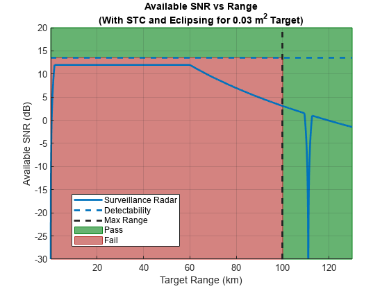
After adding the STC factor, the plot shows that the 1 m$${}^2$$ RCS target is still detected everywhere up to the maximum range $$R_m$$, while a small target with RCS of 0.03 m$${}^2$$ will not be able to reach the required $$P_d$$ of 0.9 at any range and thus will be rejected.

SNRsmallRCS = radareqsnr(lambda,R,Pt,tau,'Gain',G,'Ts',Ts,'RCS',0.03,'CustomFactor',Fecl+Fstc,'Loss',L);

radarmetricplot(R*1e-3,SNRsmallRCS,DN, ...
    'MetricName','Available SNR', ...
    'RequirementName','Detectability', ...
    'MaxRangeRequirement',Rm*1e-3, ...
    'RangeUnit','km','MetricUnit','dB', ...
    'ShowStoplight',true, ...
    'RadarName',{'Surveillance Radar'});
title([{'Available SNR vs Range'}, {'(With STC and Eclipsing for 0.03 m^2 Target)'}]);
legend('Location','best');
ylim([-30 20])

It is clear from these plots that the STC only scales the available SNR up to the specified cutoff range and does not affect the available SNR at the maximum range of interest.

Scanning

A radar system can scan a search volume either by mechanically rotating the antenna or by using the phased array antenna and performing electronic scanning. An imperfect shape of the antenna beam and the process of sweeping the beam across a search volume introduces additional losses to the system.

Beam Shape Loss

The radar equation uses a peak value of the antenna gain assuming each received pulse has the maximum amplitude. In reality, as the beam passes the target, the received pulses are modulated by the two-way pattern of the scanning antenna resulting in beam shape loss. Computing the exact value of this loss would require knowing the exact antenna pattern. This information might not be available in the early stages of the radar system design when this type of analysis is usually performed. Instead, the shape of the main lobe of a typical practical antenna can be well approximated by a Gaussian shape. Assuming that the radar system performs dense sampling in the spatial domain (the beam moves by less than 0.71 of the half power beamwidth), calculate the beam shape loss for one dimensional scanning.

Lb = beamloss

Lb = 
1.2338

The beam shape loss is doubled if the radar system scans in both azimuth and elevation.

beamloss(true)

ans = 
2.4677

Scan Sector Loss

In this example we assume the radar system employs an electronically steered phased array to perform scanning. Using the phased array antenna will cause an increase in the required SNR due to two effects: 1) beam broadening due to the reduced projected array area in the beam direction, and 2) reduction of the effective aperture area of the individual array elements at off-broadside angles. To account for these effects, add the scan sector loss to the detectability factor. Assume that the system in the example scans only in the azimuth dimension and the scan sector spans from –60 to 60 degrees. Compute the resultant loss.

theta = [-60 60];
Larray = arrayscanloss(Pd,Pfa,N,theta,'Swerling1')

Larray = 
2.7745

Signal Processing

Prior to detection the received radar echoes must pass through the radar signal processing chain. The purpose of different components in the signal processing chain is to guarantee the required probabilities of detection and false alarm, reject unwanted echoes from clutter, and account for variable or non-Gaussian noise. We further consider several components of the signal processing loss that must be accounted for in a surveillance radar system.

MTI

Moving target indicator (MTI) is a process of rejecting fixed or slowly moving clutter while passing echoes from targets moving with significant velocities. Typical MTI uses 2, 3, or 4-pulse canceller that implements a high-pass filter to reject echoes with low Doppler shifts. Passing the received signal through the MTI pulse canceller introduces correlation between the noise samples. This in turn reduces the total number of independent noise samples available for integration resulting in MTI noise correlation loss. Additionally, the MTI canceller significantly suppresses targets with velocities close to the nulls of its frequency response causing an additional MTI velocity response loss. Assuming a 2-pulse canceller is used, calculate these two components of the MTI loss.

m = 2;
[Lmti_a, Lmti_b] = mtiloss(Pd,Pfa,N,m,'Swerling1')

Lmti_a = 
1.4468

Lmti_b = 
8.1562

In a system that uses a single PRF, the MTI velocity response loss can be very high for the high required probability of detection. To eliminate this loss, PRF diversity is almost always used in real radar systems.

Binary Integration

Binary integration is a suboptimal noncoherent integration technique also known as the M-of-N integration. If $$M$$ out of $$N$$ received pulses exceed a predetermined threshold, a target is declared to be present. The binary integrator is a relatively simple automatic detector and is less sensitive to the effects of a single large interference pulse that might exist along with the target echoes. Therefore, the binary integrator is more robust when the background noise or clutter is non-Gaussian. Since the binary integration is a suboptimal technique, it results in a binary integration loss compared to optimal noncoherent integration. The optimal value of $$M$$ is not a sensitive selection and it can be quite different from the optimum without significant penalty resulting in the binary integration loss being lower than 1.4 dB. Calculate the binary integration loss when $$N$$ is 10 and $$M$$ is set to 6.

M = 6;
Lbint = binaryintloss(Pd,Pfa,N,M)

Lbint = 
1.0549

The binaryintloss function computes the loss assuming a steady (Swerling 0) target. Since the fluctuation loss is included in the detectability factor, the same binary integration loss computation can be used in the case of a fluctuating target.

CFAR

Constant false alarm rate (CFAR) detector is used to maintain an approximately constant rate of false target detections when the noise or the interference levels vary. Since CFAR averages a finite number of reference cells to estimate the noise level, the estimates are subject to an error which leads to a CFAR loss. CFAR loss is an increase in the SNR required to achieve a desired detection performance using CFAR when the noise levels are unknown compared to a fixed threshold with a known noise level. Calculate the CFAR loss assuming that total 120 cells are used for cell-averaging CFAR.

Nrc = 120;
Lcfar = cfarloss(Pfa,Nrc)

Lcfar = 
0.2500

Effective Detectability Factor

The scanning and the signal processing losses increase the detectability factor, which means that more energy is required to make a detection. The resulting detectability factor that includes effects of all these losses is called the effective detectability factor. Use the radarbudgetplot function to create a waterfall chart showing the combined effect of the computed scanning and signal processing losses on the detectability factor.

D = [D0 -Gi Lf Lmti_a+Lmti_b Lbint Lcfar Larray Lb];
radarbudgetplot(D, {'Single-pulse steady target','Pulse integration gain','Fluctuation loss'...
    'MTI loss', 'Binary integration loss', 'CFAR loss', 'Scan sector loss', 'Beam shape loss'});
title('Detectability Factor')

The resulting effective detectability factor equals 28.42 dB. By taking the scanning and the signal processing losses into account, the required SNR increases by almost 15 dB. The analysis shows that the system cannot actually meet the stated requirement of detecting a 1 m$${}^2$$ RCS target at 100 km with $$P_d$$ = 0.9 and $$P_{fa}$$ = 1e-6.

radarmetricplot(R*1e-3,SNR,sum(D), ...
    'MetricName','Available SNR', ...
    'RequirementName','Detectability', ...
    'MaxRangeRequirement',Rm*1e-3, ...
    'RangeUnit','km','MetricUnit','dB', ...
    'ShowStoplight',true, ...
    'RadarName',{'Surveillance Radar'});
title([{'Available SNR vs Range'}, {'(With STC, Eclipsing, Scanning and Signal Processing Losses)'}])
legend('Location','best')
ylim([-10 30]);

This problem can be addressed either by increasing the available SNR or decreasing the required SNR. Transmitting more power or increasing the antenna gains brings up the available SNR, while increasing the integration time lowers the required SNR. However, in some applications, a subset of the system parameters can be constrained by other requirements and thus cannot be changed. For example, if the analysis is performed for an existing system, increasing the available SNR might not be an option. In that case, making adjustments to the signal processing chain to lower the detectability factor could be an acceptable solution. To lower the required SNR, in the following sections we assume that the number of pulses $$N$$ is increased from 10 to 40.

In addition, we can change the requirements on the maximum range and the detection probabilities. Instead of a single number specifying the desired probability of detection or the maximum range, a pair of Objective and Threshold values can be defined. The Objective requirement describes the desired performance level of the system that would be needed to fully satisfy the mission needs. The Threshold requirement describes a minimum acceptable performance level of the system. Using a pair of values to define a requirement instead of a single value provides more flexibility to the design and creates a trade-space for selecting the system parameters. In this example, we assume that the Objective requirement for $$P_d$$ is 0.9 and set the Threshold value to 0.8. Similarly, the Objective maximum range requirement remains 100 km, while the Threshold value is set to 90 km. The detectability factor is now computed both for the Objective and the Threshold $$P_d$$.

N = 40;
M = 18;
Pd = [0.9 0.8];

[Lmti_a, Lmti_b] = mtiloss(Pd,Pfa,N,m,'Swerling1');
Dx = detectability(Pd,Pfa,N,'Swerling1') + cfarloss(Pfa,Nrc) + beamloss ...
    + Lmti_a + Lmti_b + binaryintloss(Pd,Pfa,N,M) + arrayscanloss(Pd,Pfa,N,theta,'Swerling1')

Dx = 2×1

   24.2522
   18.0494

Rm = [100e3 90e3];
radarmetricplot(R*1e-3,SNR,Dx(1),Dx(2), ...
    'MetricName','Available SNR', ...
    'RequirementName','Detectability', ...
    'MaxRangeRequirement',Rm*1e-3, ...
    'RangeUnit','km','MetricUnit','dB', ...
    'ShowStoplight',true, ...
    'RadarName',{'Surveillance Radar'});
title([{'Available SNR vs Range'}, {'(N=40)'}])
legend('Location','best')
ylim([-10 30]);

The SNR vs Range plot now has a yellow Warn zone indicating the SNR values and target ranges where the performance of the system is between the Objective and the Threshold requirements. We can see that up to approximately 70 km the system meets the Objective requirement for $$P_d$$. From 70 km to 100 km the Objective requirement for $$P_d$$ is violated while the Threshold requirement is still satisfied.

Effective Probability of Detection

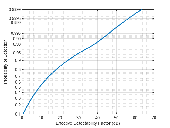
The SNR vs Range plot above shows that the detection performance of the radar system varies with range. A 1 m$${}^2$$ target at ranges below 70 km will be detected with the probability of detection greater than or equal to 0.9, while between 70 km and 100 km it will be detected with $$P_d$$ of at least 0.8. Since some of the considered losses depend on the probability of detection, the actual $$P_d$$ at the detector output varies with range. We can use the ROC curve to compute $$P_d$$ as a function of range.

% Generate a vector of probability values at which to compute the ROC curve
p = probgrid(0.1,0.9999,100);

% Compute the required SNR at these probabilities
[lmti_a, lmti_b] = mtiloss(p,Pfa,N,m,'Swerling1');
dx = detectability(p,Pfa,N,'Swerling1') + cfarloss(Pfa,Nrc) + beamloss ...
    + lmti_a + lmti_b + binaryintloss(p,Pfa,N,M) + arrayscanloss(p,Pfa,N,theta,'Swerling1');

% Plot the ROC curve
helperRadarPdVsSNRPlot(dx,p,[0.1 0.9999]);

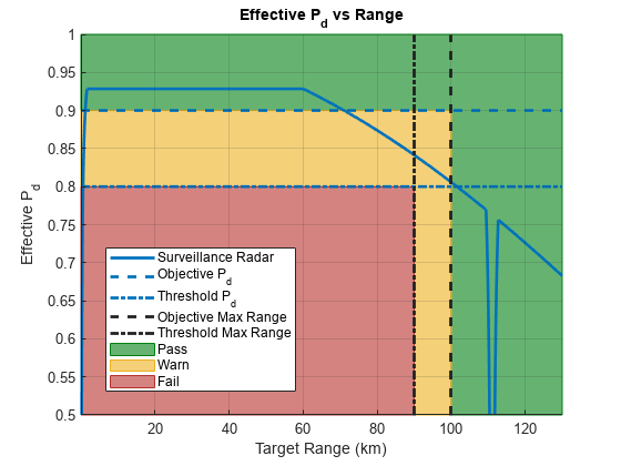
The effective probability of detection at the detector output can now be computed by interpolating this ROC curve at the available SNR values.

% Interpolate the ROC curve at the available SNR
Pdeff = rocinterp(dx,p,SNR,'snr-pd');

% Plot the effective Pd as a function of range
radarmetricplot(R*1e-3,Pdeff,Pd(1),Pd(2), ...
    'MetricName','Effective P_d', ...
    'RequirementName','P_d', ...
    'MaxRangeRequirement',Rm*1e-3, ...
    'RangeUnit','km', ...
    'ShowStoplight',true, ...
    'RadarName',{'Surveillance Radar'});
legend('Location','best')
ylim([0.5 1.0])

This result shows that due to application of the STC the probability of detection is almost constant for ranges from 2 km to 60 km. For a target with 1 m$${}^2$$ RCS it is higher than 0.92. In the range between 70 km and 87 km the effective $$P_d$$ is above 0.85. At the Threshold value of the maximum range requirement the probability of detection is approximately 0.84, and at the Objective range of 100 km it is slightly above 0.8.

Summary

This example shows how various losses impact the detection performance of a radar system. It starts with a radar equation and introduces the concepts of the available SNR and the detectability factor. Considering an example surveillance radar system, it shows how the available SNR is reduced by STC and eclipsing, while the detectability factor is increased by scanning and signal processing losses. Finally, the example demonstrates how to compute the effective probability of detection at the receiver output for different target ranges.

References

1. Barton, D. K. Radar equations for modern radar. Artech House, 2013.

2. Richards, M. A., Scheer, J. A. & Holm, W. A. Principle of Modern Radar: Basic Principles. SciTech Publishing, 2010.