Reconstruct Phase Space
Reconstruct phase space of a uniformly sampled signal in the Live Editor
Description
The Reconstruct Phase Space task lets you interactively reconstruct phase space of a uniformly sampled signal. The task automatically generates MATLAB® code for your live script. For more information about Live Editor tasks generally, see Add Interactive Tasks to a Live Script.
Phase space reconstruction is useful to verify the system order and reconstruct all
dynamic system variables, while preserving system properties. Reconstructing the phase space
is performed when limited data is available, or when the phase space dimension and lag values
are unknown. Also, the nonlinear features approximateEntropy, correlationDimension, and lyapunovExponent use phase space reconstruction as the first step of the
computation. For more information about phase space reconstruction, see phaseSpaceReconstruction.
Open the Task
To add the Reconstruct Phase Space task to a live script in the MATLAB Editor:
On the Live Editor tab, select Task > Reconstruct Phase Space.
In a code block in your script, type a relevant keyword, such as
phaseorphase space. SelectReconstruct Phase Spacefrom the suggested command completions.
Examples
Use the Reconstruct Phase Space task in the Live Editor to interactively reconstruct the phase space of a uniformly sampled signal. Experiment with different values for lag, embedding dimension, histogram bins and distance threshold. The task automatically generates code reflecting your selections.
For this example, consider 'uavPositionData.mat' which contains signal xv which is the x-component of a 3-D path traversed by an unmanned aerial vehicle (UAV). The x, y, and z coordinates define a circle of 2-m radius at 0.75-m altitude.
load('uavPositionData.mat','xv')
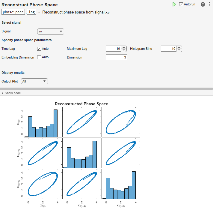
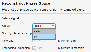
To reconstruct the phase space of the signal xv, open the Reconstruct Phase Space task in the Live Editor. On the Live Editor tab, select Task > Reconstruct Phase Space. In the task, select signal xv.
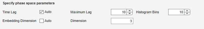
Clear the Time Lag check box if you want to use your own values in the Maximum Lag and Histogram Bins fields. For this example, leave the box checked to calculate the lag using Average Mutual Information (AMI). Since dimension is known, clear the Embedding Dimension field and specify dimension as 3.
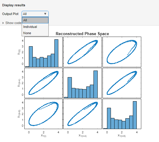
Evaluate whether the reconstructed phase space preserves the system dynamics with the assigned values by observing the output plots. You can toggle between the display type by choosing between Individual or All in the Output Plot menu.
The task generates code in your live script. The generated code reflects the parameters and options you select, and includes code to generate the type of plot you specify. To see the generated code, click ![]() above the plot. The task expands to display the generated code.
above the plot. The task expands to display the generated code.
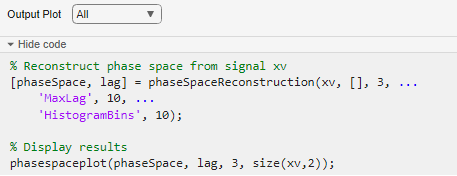
By default, the generated code uses phaseSpace as the name of the output variable. To specify a different output variable name, enter a new name in the summary line at the top of the task. For instance, change the name to pSpace.
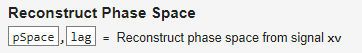
The task updates the generated code to reflect the new variable name, and the new variable pSpace appears in the MATLAB workspace. You can use the reconstructed phase space to identify condition indicators like Lyapunov exponent or correlation dimension.
Related Examples
Parameters
Version History
Introduced in R2019b