adjacentPairCorrelationModel
Identify worst cell relative to other cells in serially connected lithium-ion battery pack
Since R2023a
Syntax
Description
adjacentPairCorrelationModel( analyzes
the battery data in data)data to determine the voltage correlation
coefficients between adjacent cells in a serially connected lithium-ion battery pack, and
plots the results.
The lower the correlation coefficient is between a pair of adjacent cells, the more likely it is that one of the cells in the pair has a fault condition, such as an internal short circuit [1]. The plot legend indicates the cell pair with the lowest correlation coefficients. Using this syntax also displays the index of the worst cell in the pack.
The algorithm imposes no restrictions on battery activity during the collection of
data. The battery can be in any operating sequence, including
charging, discharging, and standby phases.
adjacentPairCorrelationModel(
incorporates additional options specified by one or more name-value arguments. For example,
increase the data,Name=Value)SquarewaveAmp argument to a value greater than the default
value of 0.003 to accommodate higher levels of noise when the batteries are at rest.
Examples
Load the data, which represents an operating profile for an eight-cell battery pack in which one cell is experiencing an internal short circuit. The profile includes standby, driving, charging, and balancing phases. The data consists of 10 columns that contain the sample time (column 1), battery voltages (columns 2–9), and pack current (column 10).
load internalShortCircuit.mat internalShortCircuit
For the adjacent-pair correlation model, you need only the cell voltages. Extract the voltage columns into the data set data.
data = internalShortCircuit(:,2:end-1);
Plot the battery voltages.
plot(data)
legend('Voltages (V)')
title('InternalShortCircuit Dataset - Voltages')
ylabel('Voltage (V) Values')
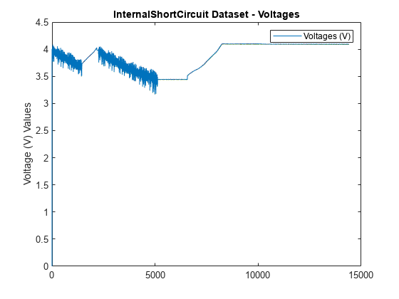
The voltages appear to track closely, but at this scale it is hard to differentiate them.
Zoom into the region after t = 4000 to show the individual voltages more clearly.
xlim([4000 4010])
ylim([3.4 3.6])
title('Voltage Separation')
ylabel('Voltages (V)')
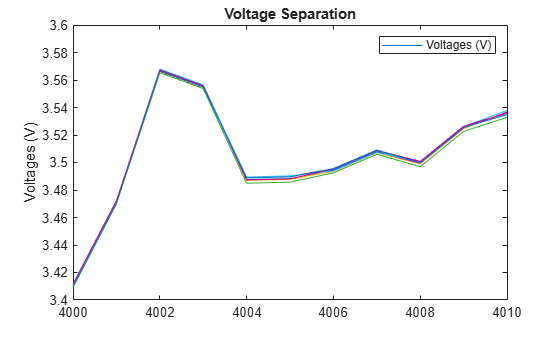
The voltages track closely together. There is no cell that is obviously degrading relative to the others.
Identify the worst cell using adjacentPairCorrelationModel.
adjacentPairCorrelationModel(data)
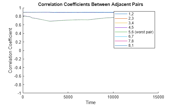
ans =
5
The correlation model identifies cell pair 5,6 as the worst pair and cell 5 as the worst cell.
Load the data, which is contained in a table, and show the first two rows.
load internalShortCircuitTbl.mat internalShortCircuitTbl
head(internalShortCircuitTbl,2)
    Time    Cell1     Cell2     Cell3    Cell4     Cell5     Cell6     Cell7     Cell8    Current
    ____    ______    ______    _____    ______    ______    ______    ______    _____    _______

     0           0         0        0         0         0         0         0        0       0
     5      4.0037    4.0018    4.002    4.0012    4.0029    4.0012    4.0042    4.002       0
The adjacent-pair correlation model does not require the Current values. Extract the time and voltage values into the timetable data.
data = internalShortCircuitTbl(:,1:end-1);
head(data,2)
    Time    Cell1     Cell2     Cell3    Cell4     Cell5     Cell6     Cell7     Cell8
    ____    ______    ______    _____    ______    ______    ______    ______    _____

     0           0         0        0         0         0         0         0        0
     5      4.0037    4.0018    4.002    4.0012    4.0029    4.0012    4.0042    4.002
Use adjacentPairCorrelationModel to identify the worst cell. Use Time to specify the time variable.
adjacentPairCorrelationModel(data(:,2:end),Time=data.Time)
ans =
5
The function identifies the worst pair and the worst cell within the pair.
Load the data, which is contained in a timetable, and extract the cell voltages into data.
load internalShortCircuitTT.mat internalShortCircuitTT
data = internalShortCircuitTT(:,1:end-1);
Run adjacentPairCorrelationModel using output arguments to store the analysis results.
[worstcell,corrcoef] = adjacentPairCorrelationModel(data);
Identify the worst cell.
iwc = worstcell
iwc =
5
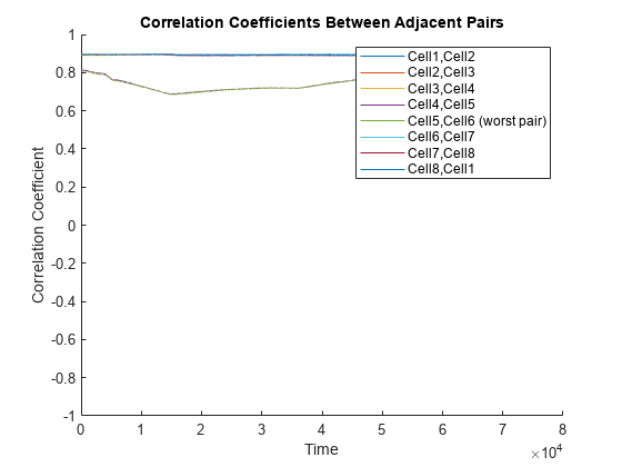
Plot the estimated correlation coefficient curves. For the legend, use the VariableNames property of data to access the cell names. With this plotting approach, the curve for each cell in the legend represents the correlation coefficient curve between that cell and the cell to the right in data.
For example, Cell1 represents the correlation curve between Cell1 and Cell2. Cell8 represents the correlation curve between Cell8 and Cell1.
plot(corrcoef.Time,corrcoef.Variables)
title('Correlation Coefficient Curves')
legend(corrcoef.Properties.VariableNames)
ylabel('corrcoef')
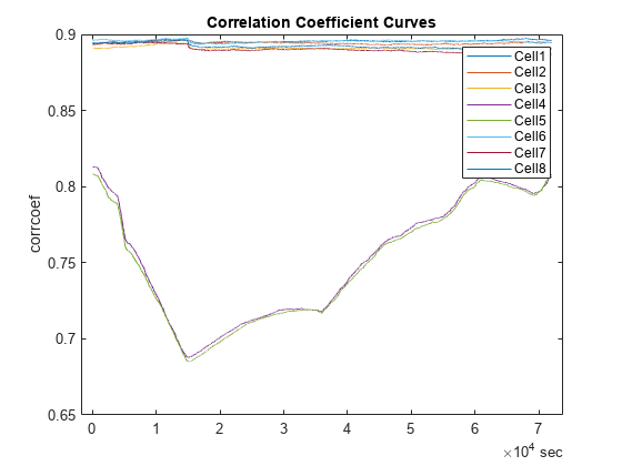
Cell 5, which the function identifies as the worst cell, has the lowest pair of correlation coefficient curves.
Input Arguments
Name-Value Arguments
Output Arguments
References
[1] Xia, Bing, Yunlong Shang, Truong Nguyen, and Chris Mi. “A Correlation Based Fault Detection Method for Short Circuits in Battery Packs.” Journal of Power Sources 337 (January 2017): 1–10. https://doi.org/10.1016/j.jpowsour.2016.11.007.
Extended Capabilities
Version History
Introduced in R2023a