Accelerate Solving Linear Equations Using GPU

This example shows how to speed up solving systems of linear equations using a GPU.

In this example, you solve a system of linear equations using the CPU and the GPU and compare the speed of CPU and GPU execution. On the GPU, you also solve the system using both full and sparse gpuArray input. Using sparse arrays to store matrices that contain many zeros can reduce memory requirements.

Systems of Linear Equations

An important problem in technical computing is how to efficiently solve systems of simultaneous linear equations. In matrix notation, you can write a system of simultaneous linear equations as

$Ax = b$ .

Although it is not standard mathematical notation, MATLAB® uses the division terminology familiar in the scalar case to describe the solution of a general system of simultaneous equations. The backslash symbol, \, corresponds to the MATLAB function mldivide. This operator is used to denote the solution to the matrix equations $Ax = b$ , obtained using mldivide:

$x = A \ b$ .

Most linear systems involve a square coefficient matrix A, and a single right-hand side column vector b.

Define Problem

This figure depicts a plane truss having 13 members (the numbered lines) connecting 8 evenly-spaced joints (the numbered circles) [1]. The indicated loads of 10, 15, and 20 tons are applied at joints 2, 5, and 6, respectively, and the goal is to determine the resulting force on each member of the truss.

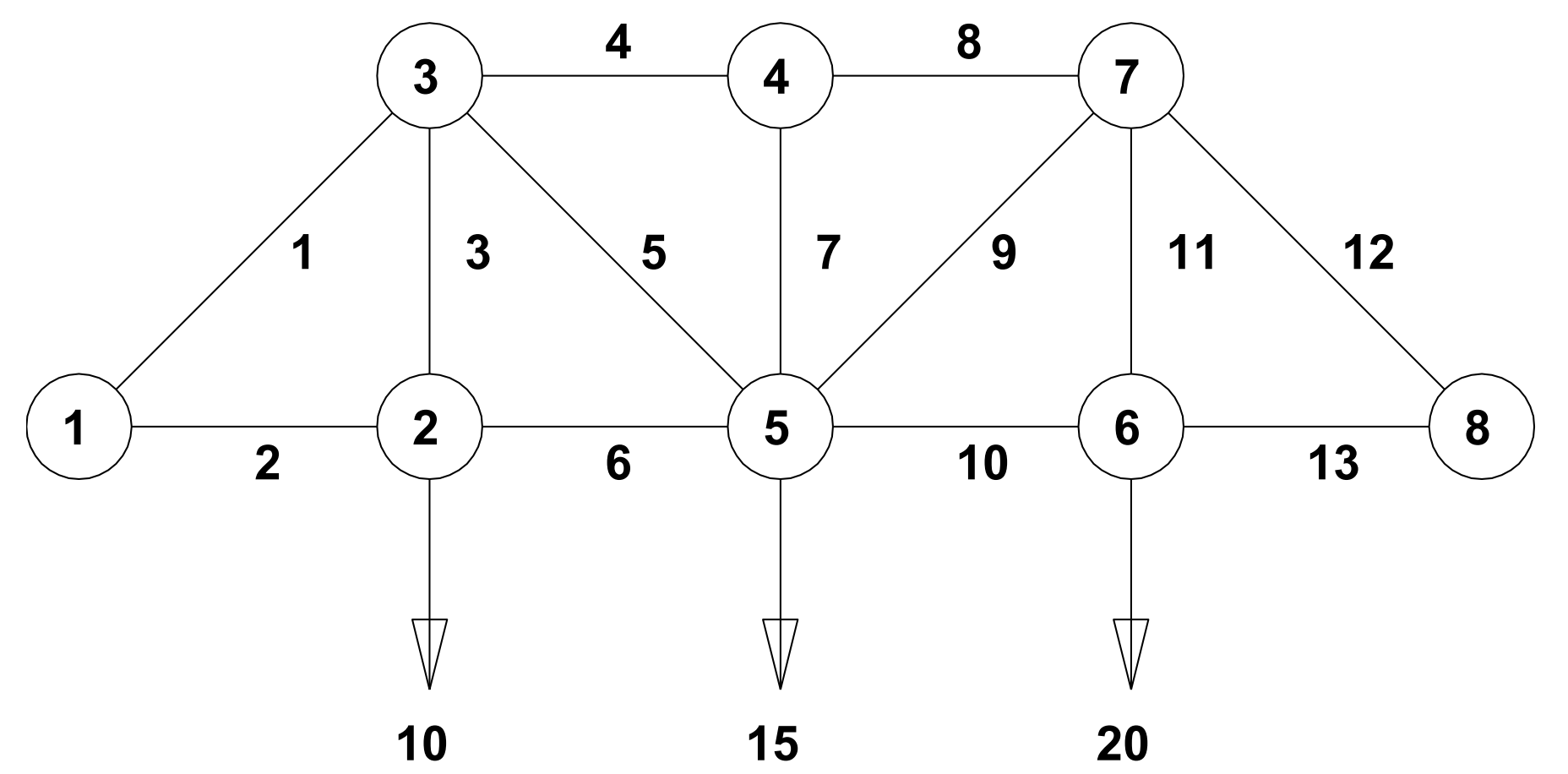
Plane truss with 13 members connected by 8 joints.

For the truss to be in static equilibrium, there must be no net force, horizontally or vertically, at any joint. Thus, you can determine the member forces by equating the horizontal forces to the left and right at each joint, and similarly equating the vertical forces upward and downward at each joint. For the eight joints, this would give 16 equations, which is more than the 13 unknown factors to be determined. For the truss to be statically determinate, that is, for there to be a unique solution, assume that joint 1 is rigidly fixed both horizontally and vertically and that joint 8 is fixed vertically. By resolving the member forces into horizontal and vertical components and defining $α = \frac{1}{\sqrt{2}}$ , you can obtain the following system of equations for the member forces $f_{i}$ :

Joint	Forces
2	$f_{2} = f_{6}$ $f_{3} = 10$
3	$α f_{1} = f_{4} + α f_{5}$ $α f_{1} + f_{3} + α f_{5} = 0$
4	$f_{4} = f_{8}$ $f_{7} = 0$
5	$α f_{5} + f_{6} = α f_{9} + f_{10}$ $α f_{5} + f_{7} + α f_{9} = 15$
6	$f_{10} = f_{13}$ $f_{11} = 20$
7	$f_{8} + α f_{9} = α f_{12}$ $α f_{9} + f_{11} + α f_{12} = 0$
8	$f_{13} + α f_{12} = 0$

To allow you to solve for x in MATLAB, where x is a column vector of forces $f_{2}$ to $f_{12}$ , first use the force equations to define the matrix A and the column vector of loads b. The rows of A and b correspond to the force equations in the table above.

a = 1/sqrt(2);

A = [0 1 0 0 0 -1 0 0 0 0 0 0 0; ...
    0 0 1 0 0 0 0 0 0 0 0 0 0; ...
    a 0 0 -1 -a 0 0 0 0 0 0 0 0; ...
    a 0 1 0 a 0 0 0 0 0 0 0 0; ...
    0 0 0 1 0 0 0 -1 0 0 0 0 0; ...
    0 0 0 0 0 0 1 0 0 0 0 0 0; ...
    0 0 0 0 a 1 0 0 -a -1 0 0 0; ...
    0 0 0 0 a 0 1 0 a 0 0 0 0; ...
    0 0 0 0 0 0 0 0 0 1 0 0 -1; ...
    0 0 0 0 0 0 0 0 0 0 1 0 0; ...
    0 0 0 0 0 0 0 1 a 0 0 -a 0; ...
    0 0 0 0 0 0 0 0 a 0 1 a 0; ...
    0 0 0 0 0 0 0 0 0 0 0 a 1];

b = [0 10 0 0 0 0 0 15 0 20 0 0 0]';

Solve Equation

Use the mldivide function (the \ operator) to solve for x. To minimize computation time, MATLAB uses different algorithms depending on the properties of matrix A.

x = A\b

Before you compute x using a GPU, first check that you have a supported GPU.

gpu = gpuDevice;
disp(gpu.Name + " GPU selected.")

NVIDIA RTX A5000 GPU selected.

Convert matrix A to a gpuArray. This moves the data to GPU memory. Many MATLAB linear algebra functions, including mldivide, run on a GPU if the input data is a gpuArray. If a function supports gpuArray input, this is indicated in the Extended Capabilities section of the function reference page.

A = gpuArray(A);

Solve for x on the GPU. The output is also a gpuArray.

x = A\b;

Verify that the calculated solution accurately reconstructs the vector b.

A*x

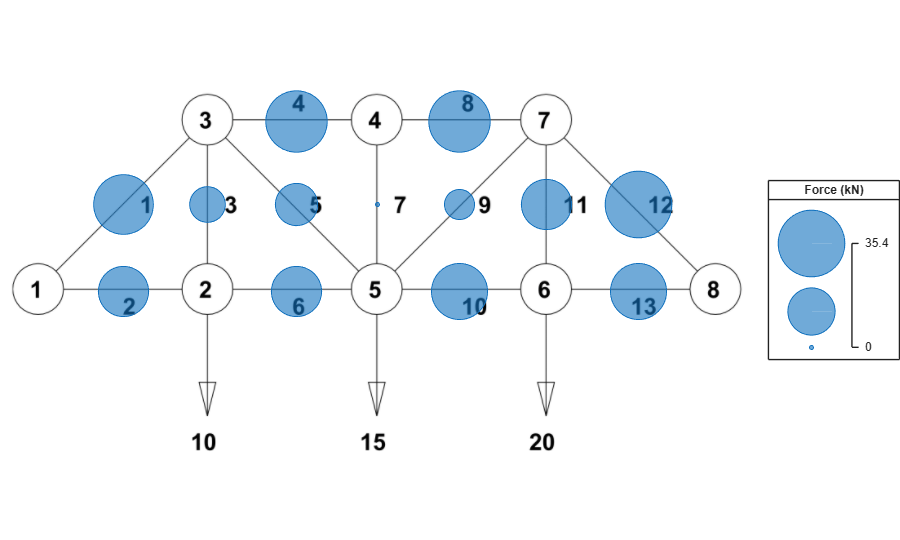
Overlay the calculated forces on the truss members using the plotTrussForces function. This function is attached to the example as a supporting file.

plotTrussForces(x)

Compare the CPU and GPU execution times using the timeit and gputimeit functions respectively. gputimeit is preferable to timeit for functions that use the GPU, because it ensures that all operations on the GPU have finished before recording the time and compensates for the overhead. However, timeit offers greater precision for operations that do not use a GPU.

A = gather(A);
tCPU = timeit(@() A\b,1)

tCPU = 
3.2756e-06

A = gpuArray(A);
tGPU = gputimeit(@() A\b,1)

tGPU = 
0.0013

disp("Speedup of CPU over GPU for a small problem: " + round(tGPU/tCPU,1) + "x")

Speedup of CPU over GPU for a small problem: 387.6x

Scale Up

For a system with eight joints and a 13-by-13 matrix A, the CPU solves the system significantly faster than the GPU. This is expected, as GPUs have many cores and therefore excel only when operating on large amounts of data.

To show the scale at which GPU computing can be effective, define a larger problem. Use the trussMatrix and randomLoad functions to generate a matrix A and column vector b that represents the forces and loads on a plane truss with 1000 joints. These functions are attached to the example as supporting files.

A = trussMatrix(1000);
b = randomLoad(1000,30);

Compare the CPU and GPU execution times.

tCPU = timeit(@() A\b,1)

tCPU = 
0.0638

A = gpuArray(A);
x = A\b;
tGPU = gputimeit(@() A\b,1)

tGPU = 
0.0246

disp("Speedup of GPU over CPU for a large problem: " + round(tCPU/tGPU,1) + "x")

Speedup of GPU over CPU for a large problem: 2.6x

Verify that the calculated solution accurately reconstructs the vector b. Because the vectors are large, compare only the first 10 elements.

bCheck = A*x;
[b(1:10) bCheck(1:10)]

ans =

         0         0
   19.0000   19.0000
         0         0
         0         0
         0   -0.0000
         0         0
         0    0.0000
   18.0000   18.0000
         0         0
   17.0000   17.0000

Exploit Matrix Sparsity

As the numbers of joints increases, the sparsity of the matrix A increases; that is, the percentage of elements that are zero increases. Calculate the density of matrix A. Only about 0.01% of the elements are nonzero.

density = nnz(A)/numel(A)

density = 
0.0013

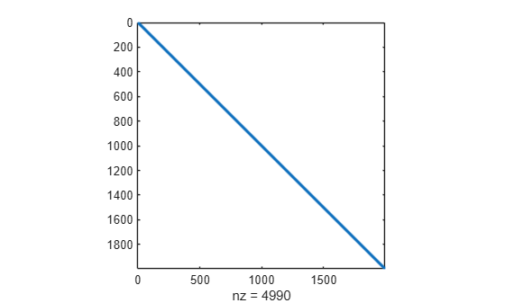
Plot the sparsity pattern of matrix A. Most of the nonzero elements are close to the main diagonal.

figure
spy(A)

Sparse arrays in MATLAB provide efficient storage of matrices with a large percentage of zeros. While full (or dense) matrices store every single element in memory regardless of value, sparse matrices store only the nonzero elements and their locations. For this reason, using sparse matrices can significantly reduce the amount of memory required for data storage. For more information, see Computational Advantages of Sparse Matrices and Work with Sparse Arrays on a GPU.

Convert matrix A into a sparse matrix and compare the size of the matrix when stored in full versus sparse form. The degree of reduction in required memory depends on the size and structure of the matrix.

sparseA = sparse(A);
whos A sparseA

  Name            Size                 Bytes  Class       Attributes

  A            1997x1997            31904072  gpuArray              
  sparseA      1997x1997               67872  gpuArray    sparse

Time solving the system with sparse gpuArray input. Many of the functions that can solve linear systems in MATLAB support sparse arrays, including mldivide.

tGPUSparse = gputimeit(@() sparseA\b,1)

tGPUSparse = 
0.0278

References

[1] Moler, Cleve B. Numerical Computing with MATLAB. Society for Industrial and Applied Mathematics, 2004. https://doi.org/10.1137/1.9780898717952.