Reverse-Capable Motion Planning for Tractor-Trailer Model Using plannerControlRRT
This example shows how to find global path-planning solutions for systems with complex kinematics using the kinematics-based planner, plannerControlRRT. The example is organized into three primary sections:
Introduction to Kino-Dynamic Planning.
Adapting
plannerControlRRTto a Tractor-Trailer System.Finding Collision-Free Trajectories Using a Kinematic System.
Introduction to Kino-Dynamic Planning
Planner Description
Conventional geometric planners, such as RRT, RRT*, and hybridA*, are fast and extensible algorithms capable of finding complete and optimal solutions to a wide variety of planning problems. One trade-off, however, is that they make assumptions about the planning space that may not hold true for a real-world system. Conventional geometric planners assume that any two states in a space can be connected by a trajectory with no residual error, and that the paths returned by the geometric planner can be tracked by the physical system.
For systems with complex kinematics, or those that do not have easily determined closed-form solutions for connecting states, use kino-dynamic planners, such as plannerControlRRT. Kino-dynamic planners trade completeness for planning flexibility, and leverage a system's own kinematic model and controller to generate feasible and trackable trajectories.
To plan for a given system, the plannerControlRRT feature requires this information:
A utility to sample states in the planning space.
A metric to estimate the cost of connecting two states.
A mechanism to deterministically propagate the system from one state toward another.
A utility to determine whether a state has reached the goal.
This example demonstrates how to formulate these different utilities for a tractor-trailer system and adapt them into the planning infrastructure. This preview shows the result:
% Attempt to generate MEX to accelerate collision checking
genFastCC
Code generation successful.
% load preplannedScenarios
parkingScenario = load("parkingScenario.mat");
planner = parkingScenario.planner;
start   = parkingScenario.start;
goal    = parkingScenario.goal;

% Display the scenario and play back the trajectory
show(planner.StatePropagator.StateValidator);
axis equal
hold on
trajectory = plan(planner,start,goal);
demoParams = trajectory.StatePropagator.StateSpace.TruckParams;
exampleHelperPlotTruck(demoParams,start); % Display start config
exampleHelperPlotTruck(demoParams,goal);  % Display goal config

% Plan path using previously-built utilities
rng(1)
trajectory = plan(planner,start,goal);

% Animate the trajectory
exampleHelperPlotTruck(trajectory);
hold off
Kino-Dynamic Planning Algorithm
If you are already familiar with geometric planners, an iteration of the plannerControlRRT search algorithm should look familiar, but with a few extra steps:
Sample a target state.
Find the approximate nearest neighbor to the target state in the search tree.
Generate a control input (or reference value) and control duration that drives the system toward the target.
Propagate (extend) the system towards the sample while validating intermediate states along the propagated trajectory. Return the valid sequence of states, controls, and durations.
Check whether any returned states have reached the goal.
If the goal has been found, exit. Otherwise add the final state, initial control, cumulative duration, and target to the tree.
(Optional) Sample a goal-configuration and control and repeat steps 4,5, and 6 the desired number of times.
Components Required by plannerControlRRT Framework
To adapt the planner to a specific problem, you must implement custom nav.StatePropagator and nav.StateSpace classes. The section below maps the steps described in the Kino-Dynamic Planning Algorithm section to the class and method responsible:
plannerControlRRTchecks whether any returned states have reached the goal.By default, exiting planning or adding to the search tree is performed by the
distancefunction of the propagator. You can override it by supplying the planner with a function handle during construction.By default, each time the planner successfully adds a node to the tree, it will attempt to propagate this newly added state towards the goal-configuration. This goal-propagation can occur multiple times in a row, or disabled entirely, by modifying the
NumGoalExtensionproperty of the planner.
For more detailed function syntax, argument requirements, and examples, see plannerControlRRT, nav.StateSpace, and nav.StatePropagator.
Adapting plannerControlRRT to a Truck-Trailer System
This section demonstrates how to formulate, model, and control a two-body truck-trailer system. This system is inherently unstable during reverse motion, so paths returned by conventional geometric planners are unlikely to produce good results during path following. To accurately model this system, you must:
Define a state transition function.
Define the geometric model parameters.
Create a control law attuned to the parameterized model.
Create a distance heuristic attuned to the parameterized model.
Package the kinematic model, distance metric, and control law inside a custom state space and state propagator.
Plan a path for several problem scenarios.
Define State Transition Function
This tractor-trailer system is comprised of two rigid bodies connected at a kingpin hitch, which is modeled as a revolute joint. The trailer body makes contact with the ground at the rear axle, and the front of the trailer is supported by the hitch, located somewhere along the axial centerline of the truck.
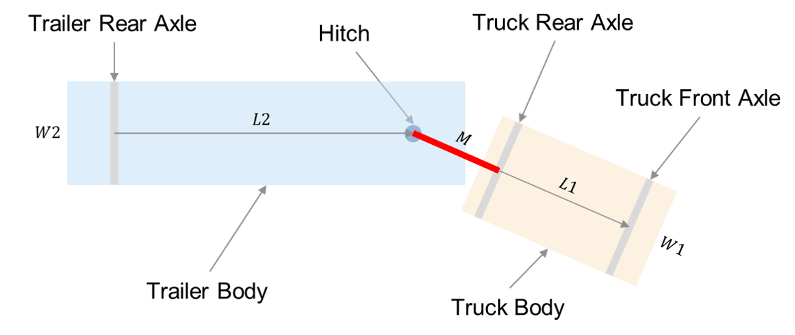
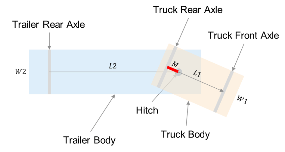
Trailing Configuration (left, M < 0), OverCenter Configuration (right, M > 0)
Use the geometric configuration for a two-body truck-trailer system from the Truck and Trailer Automatic Parking Using Multistage Nonlinear MPC example, expressed as:
,
where:
— Global -position of the center of the trailer rear axle.
— Global -position of the center of the trailer rear axle.
— Global angle of the trailer orientation, where
0is east.— Truck Orientation with respect to the trailer, where
0is aligned.
For planning purposes, append a direction flag, , and the total distance traveled from the start configuration, to the state vector, for the final state notation:
— Indicates the desired control mode (forward or reverse) or a required velocity, ensuring the system propagates toward the goal occur in a desired direction.
— Modifies the behavior of the propagator's
distancefunction of the propagator. You can modify the propagator'sTravelBiasproperty to change the frequency with which the nearest-neighbor comparison includes or excludes the root-to-node cost. Values closer to 0 result in a faster search of the planning space, at the expense of more locally optimal connections being made. Values closer to 1 can improve planner solutions, but increase planning time.
This state transition function is an extension of TruckTrailerStateFcn. For a full derivation of the state transition function, see exampleHelperStateDerivative, which is a simplification of this N-trailer model [1]:
For simplicity, this model treats as the instantaneous velocity and steering angle command applied to the system, generated by a higher-level controller. For more information, see Create Control Laws for Stable Forward and Reverse Motion.
Define Geometric Model Parameters and Demonstrate Instability
The kinematic characteristics of this vehicle are heavily influenced by the choice of model parameters. Create a structure that describes a tractor-trailer system.
truckParams = struct;
truckParams.L1 = 6;     % Truck body length
truckParams.L2 = 10;    % Trailer length
truckParams.M  = 1;     % Distance between hitch and truck rear axle along truck body +X-axis
Define properties related to visualization and collision-checking.
truckParams.W1 = 2.5;               % Truck width
truckParams.W2 = 2.5;               % Trailer width
truckParams.Lwheel = 1;             % Wheel length
truckParams.Wwheel = 0.4;           % Wheel width
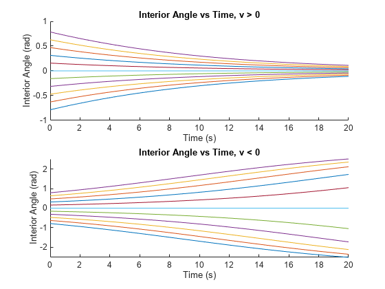
Using the exampleHelperShowOpenLoopDynamics function and specified model parameters, propagate the system state using its open-loop dynamics to demonstrate that the interior angle is self-stabilizing during forward motion, and unstable during reverse motion for any non-zero .
exampleHelperShowOpenLoopDynamics(truckParams);

Create Control Laws for Stable Forward and Reverse Motion
This example employs a multi-layer, mode-switching controller to control the truck-trailer model. At the top level, a pure pursuit controller calculates a reference point, , between a current pose, , and goal state, . The controller has two modes, for forward and reverse. For information on the basis for this control law, see [1]. For forward motion, the controller calculates a steering angle that, when held constant, drives the rear axle of the truck along an arc that intersects the reference point:
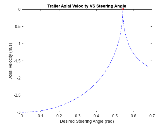
For reverse motion, the rear axle of the trailer becomes the controlled state, . Furthermore, because the system is inherently unstable during reverse motion, the control law treats the steering angle returned by the top-level controller as a reference value to a gain-scheduled LQ controller, which seeks to stabilize the interior angle of the vehicle:
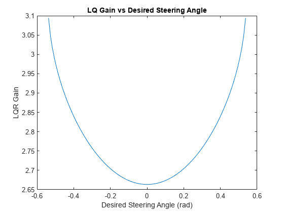
LQ Feedback Stabilization
During reverse motion, you can add a gain to the steering angle that drives the interior angle to an equilibrium point. Use the LQ controller to calculate the desired steering angle and feedback gains. The gains are the optimal solution to the Algebraic Ricatti equation, stored as a lookup table dependent on the desired steering angle. For more information about the derivation of this feedback controller, see exampleHelperCalculateLQGains:
% Define Q/R weight matrices for LQR controller
Q = 10; % Weight driving betaDot -> 0
R = 1; % Weight minimizing steering angle command

% Derive geometric steering limits and solve for LQR feedback gains
[alphaLimit, ...        % Max steady-state steering angle before jack-knife
 betaLimit, ...         % Max interior angle before jack-knife
 alphaDesiredEq, ...    % Sampled angles from stable alpha domain
 alphaGain ...          % LQ gain corresponding to desired alpha
] = exampleHelperCalculateLQGains(truckParams,Q,R);
% Add limits to the truck geometry
truckParams.AlphaLimit = alphaLimit;
truckParams.BetaLimit = betaLimit;
Specify lookahead distances for the pure pursuit controller, exampleHelperPurePursuitGetSteering, and rate and time-span information for our model simulator, exampleHelperPropagateTruck. Because reverse motion is unstable, and you have only indirect control over the interior angle, specify a larger lookahead distance in reverse. This gives the system more time to minimize the virtual steering error while maintaining a stable interior angle.
% Select forward and reverse lookahead distances. For this example,
% use a reverse lookahead distance twice as long as the forward
% lookahead distance, which itself is slightly longer than the
% wheelbase. You can tune these parameters can be tuned for
% improved performance for a given geometry.
rFWD = truckParams.L1*1.2;
rREV = rFWD*2;

% Define parameters for the fixed-rate propagator and add them to the
% control structure
controlParams.MaxVelocity = 3; % m/s
controlParams.StepSize = .1; % s
controlParams.MaxNumSteps = 50; %#ok<STRNU> % Max number of steps per propagation
Create a structure of the control-related information.
% Store gains and control parameters in a struct
controlParams = struct(...
    'MaxSteer',alphaLimit, ...          % (rad)
    'Gains',alphaGain, ...              % ()
    'AlphaPoints',alphaDesiredEq, ...   % (rad)
    'ForwardLookahead',rFWD, ...        % (m)
    'ReverseLookahead',rREV, ...        % (m)
    'MaxVelocity', 3, ...               % (m/s)
    'StepSize', 0.1, ...                % (s)
    'MaxNumSteps', 200 ...               % ()
    );
Define a Distance Heuristic
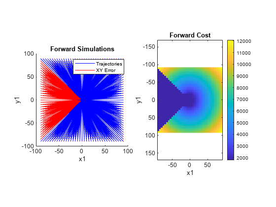
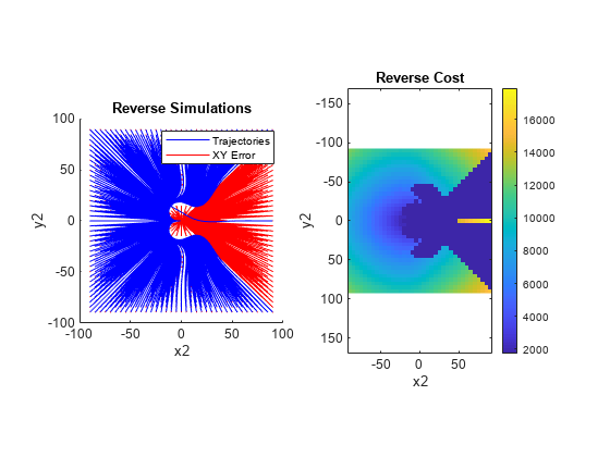
Define a distance heuristic to approximate the cost between different configurations in state-space of the system. The state propagator uses this when the planner attempts to find the nearest node in the tree to a sampled state. Calculate the cost offline using the exampleHelperCalculateDistanceMetric function, which stores it in a lookup table.
distanceHeuristic = exampleHelperCalculateDistanceMetric(truckParams,controlParams);
Adapt System for Use with Kinematic Planner
Adapt the system into a framework usable by the kinematic path-planner, plannerControlRRT. Create 3 custom classes: exampleHelperTruckStateSpace, exampleHelperTruckPropagator, and exampleHelperTruckValidator, which inherit from the nav.StateSpace, nav.StatePropagator, and nav.StateValidator subclasses, respectively.
Initialize State Space
The state-space object is primarily responsible for:
Sampling random states for the planner.
Defining and enforcing state limits within a trajectory.
Define xy- limits for the searchable region. Initialize the state-space using these limits, and the -limits determined by the geometric properties of the truck trailer.
Because the kinematic planner uses the distance function of the state-propagator for its nearest-neighbor search, leave the state-space distance method undefined. Leave the interpolate and sampleGaussian methods of the state-space similarly undefined.
% Define limits of searchable region
xyLimits = [-60 60; -40 40];

% Construct our state-space
stateSpace = exampleHelperTruckStateSpace(xyLimits, truckParams);
Initialize State Validator
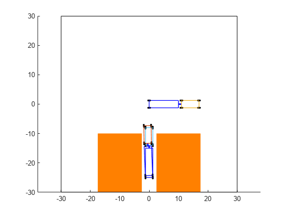
In this example, the state validator uses oriented bounding boxes (OBBs) to verify whether the vehicle is in collision with the environment. The truck is represented by two rectangles with poses defined by the state and the vehicle geometry of the truck contained in the state-space object. The environment is represented by a list of rectangles with their locations, orientations, and dimensions specified in a 1-by-N structure. Load a MAT file containing the environment into the workspace, and use the obstacles and state-space object to construct the state validator.
% Load a set of obstacles
load("Slalom.mat");

% Construct the state validator using the state space and list of obstacles
validator = exampleHelperTruckValidator(stateSpace,obstacles);
Initialize State Propagator
In kinematic planning, the state-propagator object is responsible for:
Estimating the distance between states.
Sampling initial controls to propagate over a control-interval, or capturing control inputs as reference values for lower-level controllers during propagation.
Propagating the system towards a target, and returning the valid portion of the trajectory to the planner.
For best results, the distance function should estimate the cost of the trajectory generated when propagating between states.
% Construct the state propagator using the state validator, control parameters,
% and distance lookup table
propagator = exampleHelperTruckPropagator(validator,controlParams,distanceHeuristic);
Construct Planner and Plan Path
Construct a kinematic path-planner that uses the state propagator to search for a path between the two configurations.
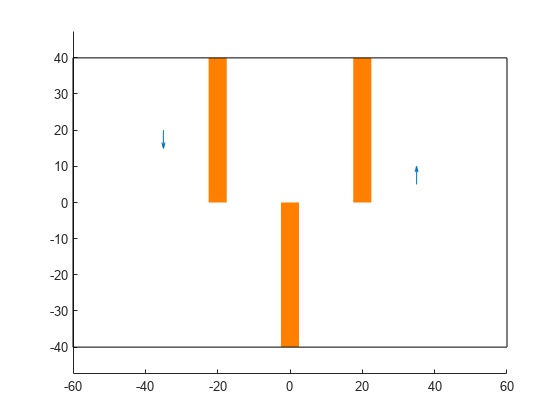
% Define start configuration
start = [35 5 pi/2 0 0 0];

% Define the goal configuration such that the truck must reverse into
% position.
goal  = [-35 20 -pi/2 0 -1 nan];

% Display the problem
figure
show(validator)
hold on
configs = [start; goal];
quiver(configs(:,1),configs(:,2),cos(configs(:,3)),sin(configs(:,3)),.1)
% Define a function to check if planner has reached the true goal state
goalFcn = @(planner,q,qTgt)exampleHelperGoalReachedFunction(goal,planner,q,qTgt);

% Construct planner
planner = plannerControlRRT(propagator,GoalReachedFcn=goalFcn,MaxNumIteration=30000);
planner.NumGoalExtension = 3;
planner.MaxNumTreeNode = 30000;
planner.GoalBias = .25;
% Search for the path
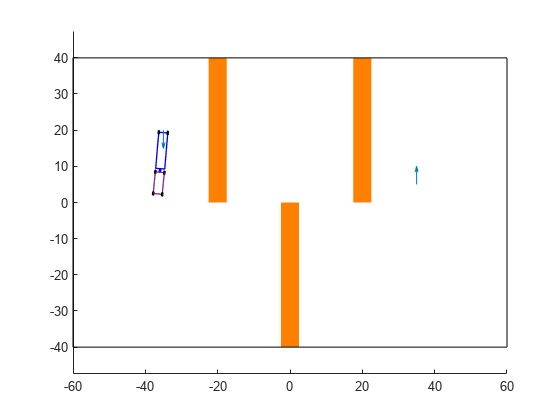
rng(0)
[trajectory,treeInfo] = plan(planner,start,goal)trajectory =
navPathControl with properties:
StatePropagator: [1×1 exampleHelperTruckPropagator]
States: [23×6 double]
Controls: [22×4 double]
Durations: [22×1 double]
TargetStates: [22×6 double]
NumStates: 23
NumSegments: 22
treeInfo = struct with fields:
     IsPathFound: 1
        ExitFlag: 1
     NumTreeNode: 2201
    NumIteration: 1196
    PlanningTime: 5.3823
        TreeInfo: [6×6602 double]
% Visualize path and waypoints
exampleHelperPlotTruck(trajectory);
hold off
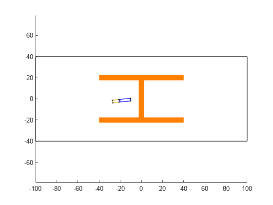
Rather than producing optimal solutions, like those generated in the Truck and Trailer Automatic Parking Using Multistage Nonlinear MPC example, the advantage of this planner lies in its ability to find viable trajectories for a wide variety of problems. In the scenario below, for instance, the generated path can be used as is, or as an initial guess for an MPC solver, helping to avoid local minima in the nonconvex problem space:
% Load scenario obstacles
nonConvexProblem = load("NonConvex.mat");

% Update validator and state space
validator.Obstacles = nonConvexProblem.obstacles;
validator.StateSpace.StateBounds(1:2,:) = [-100 100; -40 40];
figure
show(validator)

% Define start and goal
start = [10 0 0 0 NaN 0];
goal  = [-10 0 pi 0 -1 0];

% Update goal reached function
goalFcn = @(planner,q,qTgt)exampleHelperGoalReachedFunction(goal,planner,q,qTgt);
planner.GoalReachedFcn = goalFcn;

% Turn off optional every-step goal propagation
planner.NumGoalExtension = 0;

% Increase goal sampling frequency
planner.GoalBias = .25;

% Balanced search vs path optimality
propagator.TravelBias = .5;

% Plan path
rng(0)
trajectory = plan(planner,start,goal);

% Visualize result
exampleHelperPlotTruck(trajectory);
References
[1] Holmer, Olov. “Motion Planning for a Reversing Full-Scale Truck and Trailer System”. M.S. thesis, Linköping University, 2016.