Design MPC Controller for Paper Machine Process
This example shows how to design a model predictive controller for a nonlinear paper machine process using MPC Designer.
Plant Model
Ying et al. [1] studied the control of consistency (percentage of pulp fibers in aqueous suspension) and liquid level in a paper machine headbox.

The process is nonlinear and has three outputs, two manipulated inputs, and two disturbance inputs, one of which is measured for feedforward control.
The process model is a set of ordinary differential equations (ODEs) in bilinear form. The states are
H1 — Feed tank liquid level
H2 — Headbox liquid level
N1 — Feed tank consistency
N2 — Headbox consistency
The primary control objective is to hold H2 and N2 at their setpoints by adjusting the manipulated variables:
Gp — Flow rate of stock entering the feed tank
Gw — Flow rate of recycled white water
The consistency of stock entering the feed tank, Np, is a measured disturbance, and the white water consistency, Nw, is an unmeasured disturbance.
All signals are normalized with zero nominal steady-state values and comparable numerical ranges. The process is open-loop stable.
The measured outputs are H2, N1, and N2.
The Simulink® S-function, mpc_pmmodel implements the nonlinear model
equations. To view this S-function, enter the
following.
edit mpc_pmmodelTo design a controller for a nonlinear plant using MPC Designer, you must first obtain a linear model of the plant. The paper machine headbox model can be linearized analytically.
At the MATLAB® command line, enter the state-space matrices for the linearized model.
A = [-1.9300        0        0        0
      0.3940  -0.4260        0        0
           0        0  -0.6300        0
      0.8200  -0.7840   0.4130  -0.4260];
B = [1.2740   1.2740        0        0
          0        0        0        0
     1.3400  -0.6500   0.2030   0.4060
          0        0        0        0];
C = [0   1.0000        0        0
     0        0   1.0000        0
     0        0        0   1.0000];
D = zeros(3,4);
Create a continuous-time LTI state-space model.
PaperMach = ss(A,B,C,D);
Specify the names of the input and output channels of the model.
PaperMach.InputName = {'G_p','G_w','N_p','N_w'};
PaperMach.OutputName = {'H_2','N_1','N_2'};
Specify the model time units.
PaperMach.TimeUnit = 'minutes';Examine the open-loop response of the plant.
step(PaperMach)
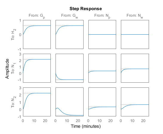
The step response shows that:
Both manipulated variables, Gp and Gw, affect all three outputs.
The manipulated variables have nearly identical effects on H2.
The response from Gw to N2 is an inverse response.
These features make it difficult to achieve accurate, independent control of H2 and N2.
Import Plant Model and Define Signal Configuration
Open the MPC Designer app.
mpcDesigner
In MPC Designer, on the MPC Designer tab, in the Structure section, click MPC Structure.
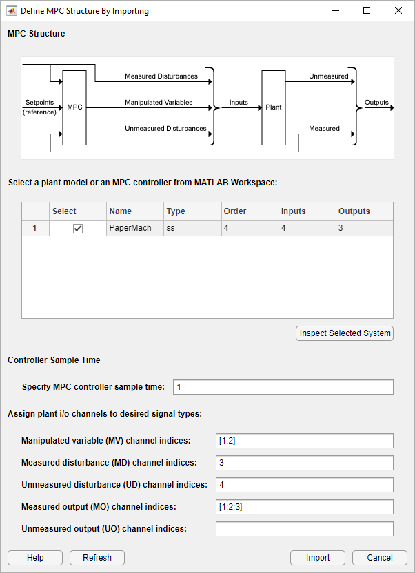
In the Define MPC Structure By Importing dialog box, select the
PaperMach plant model.
in the Specify MPC controller sample time field, enter a sample
time of 1 minute.
Assign the plant I/O channels to the following signal types:
Manipulated variables — Gp and Gw
Measured disturbance — Np
Unmeasured disturbance — Nw
Measured outputs — H2, N2, and H2
Tip
To find the correct channel indices, click Inspect Selected System to view additional model details.
Click Import.
The app imports the plant to the Data Browser and creates a default MPC controller using the imported plant.
Define Input and Output Channel Attributes
In the Structure section, select I/O Attributes.
In the Input and Output Channel Specifications dialog box, in the Unit column, define the units for each channel. Because all the signals are normalized with zero nominal steady-state values, keep the Nominal Value and Scale Factor for each channel at their default values.

Click OK to update the channel attributes and close the dialog box.
Specify Controller Sample Time and Horizons
On the Tuning tab, in the Horizon section, keep the Sample time, Prediction Horizon, and Control Horizon at their default values.
Specify Manipulated Variable Constraints
In the Design section, click Constraints.
In the Constraints dialog box, in the Input Constraints section, specify value constraints, Min and Max, for both manipulated variables.
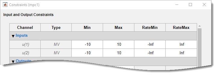
Click OK.
Specify Initial Tuning Weights
In the Design section, click Weights.
In the Weights dialog box, in the Input Weights section, increase
the Rate Weight to 0.4 for both manipulated
variables.
In the Output Weights section, specify a
Weight of 0 for the second output,
N1, and a Weight of
1 for the other outputs.
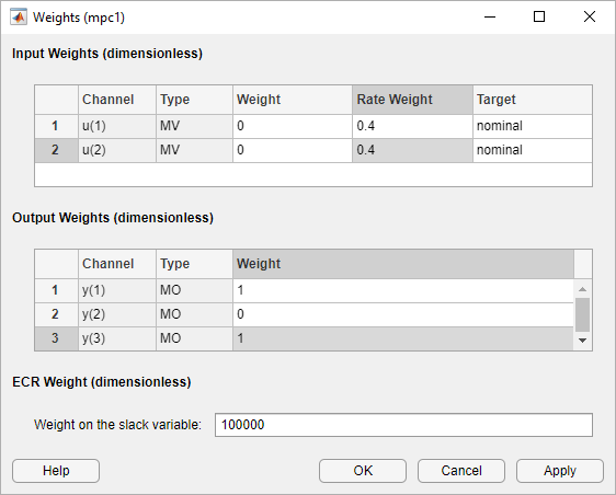
Increasing the rate weight for manipulated variables prevents overly-aggressive control actions resulting in a more conservative controller response.
Because there are two manipulated variables, the controller cannot control all three outputs completely. A weight of zero indicates that there is no setpoint for N1. As a result, the controller can hold H2 and N2 at their respective setpoints.
Click OK.
Simulate H2 Setpoint Step Response
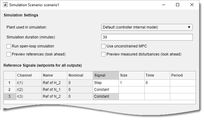
On the MPC Designer tab, in the Scenario section, click Edit Scenario > scenario1.
In the Simulation Scenario dialog box, specify a Simulation
duration of 30 minutes.
In the Reference Signals table, in the
Signal drop-down list, keep Step for the
first output. Keep the step Size at 1 and specify
a step Time of 0.
In the Signal drop-down lists for the other output reference
signals, select Constant to hold the values at their respective
nominal values. The controller ignores the setpoint for the second output since the
corresponding tuning weight is zero.
Click OK.
The app runs the simulation with the new scenario settings and updates the Input Response and Output Response plots.

The initial design uses a conservative control effort to produce a robust controller. The response time for output H2 is about 7 minutes. To reduce this response time, you can decrease the sample time, reduce the manipulated variable rate weights, or reduce the manipulated variable rate constraints.
Because the tuning weight for output N1 is
zero, its output response shows a steady-state error of about
–0.25.
Adjust Weights to Emphasize Feed Tank Consistency Control
On the Tuning tab, in the Design section, select Weights.
In the Weights dialog box, in the Output Weights section, specify
a Weight of 0.2 for the first output,
H2.
Click OK.
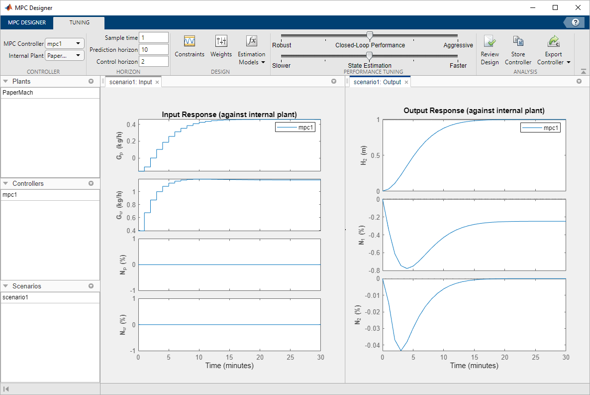
The controller places more emphasis on eliminating errors in feed tank consistency, N2, which significantly decreases the peak absolute error. The tradeoff is a longer response time of about 17 minutes for the feed tank level, H2.
Test Controller Feedforward Response to Measured Disturbances
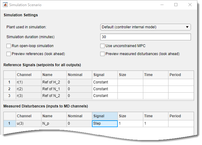
On the MPC Designer tab, in the Scenario section, click Plot Scenario > New Scenario.
In the Simulation Scenario dialog box, specify a Simulation
duration of 30 minutes.
In the Measured Disturbances table, specify a step change in
measured disturbance, Np, with a
Size of 1 and a step Time
of 1. Keep all output setpoints constant at their nominal
values.
Click OK to run the simulation and display the input and output response plots.
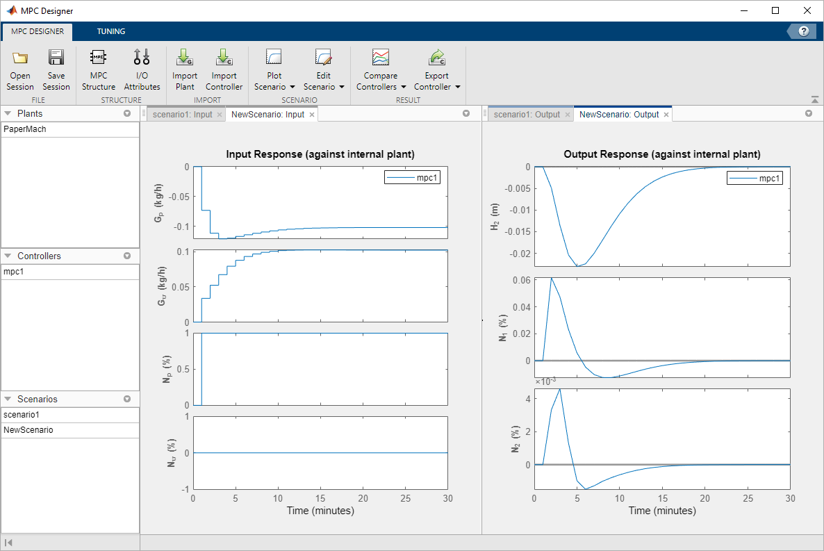
As shown in the NewScenario: Output plot, both H2 and N2 deviate little from their setpoints.
Experiment with Signal Previewing
In the Scenarios section in the lower left part of MPC
Designer, right-click NewScenario, and select
Edit.
In the Simulation Scenario dialog box, in the Simulation Settings section, check the Preview measured disturbances (look ahead) option.
Click Apply.
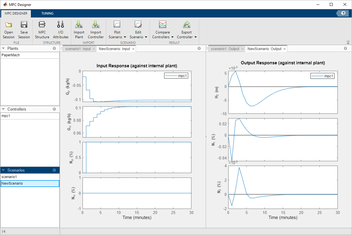
The manipulated variables begin changing before the measured disturbance occurs because the controller uses the known future disturbance value when computing its control action. The output disturbance values also begin changing before the disturbance occurs, which reduces the magnitude of the output errors. However, there is no significant improvement over the previous simulation result.
In the Simulation Scenario dialog box, clear the Preview measured disturbances option.
Click OK.
Rename Scenarios
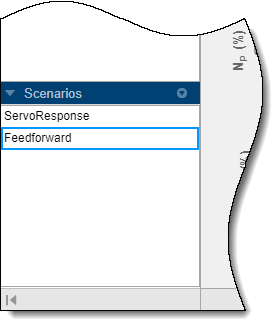
With multiple scenarios, it is helpful to provide them with meaningful names. In the Scenarios section, double-click each scenario to rename them as shown:
Test Controller Feedback Response to Unmeasured Disturbances
In the Scenarios section, right-click
FeedForward, and select Copy.
Double-click the newly created scenario, and rename it
Feedback.
Right-click the Feedback scenario, and select
Edit.
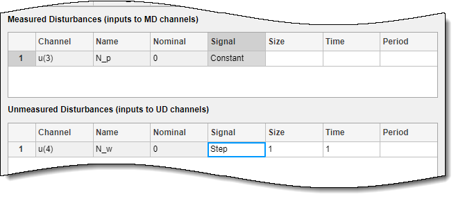
In the Simulation Scenario dialog box, in the Measured
Disturbances table, in the Signal drop-down list, select
Constant to remove the measured disturbance.
In the Unmeasured Disturbances table, in the
Signal drop-down list, select Step to
simulate a sudden, sustained unmeasured input disturbance.
Keep the step Size to 1 and the step
Time to 1.
Click OK to update the scenario settings, and run the simulation.
In the Data Browser, in the Scenarios
section, right-click Feedback, and select
Plot.
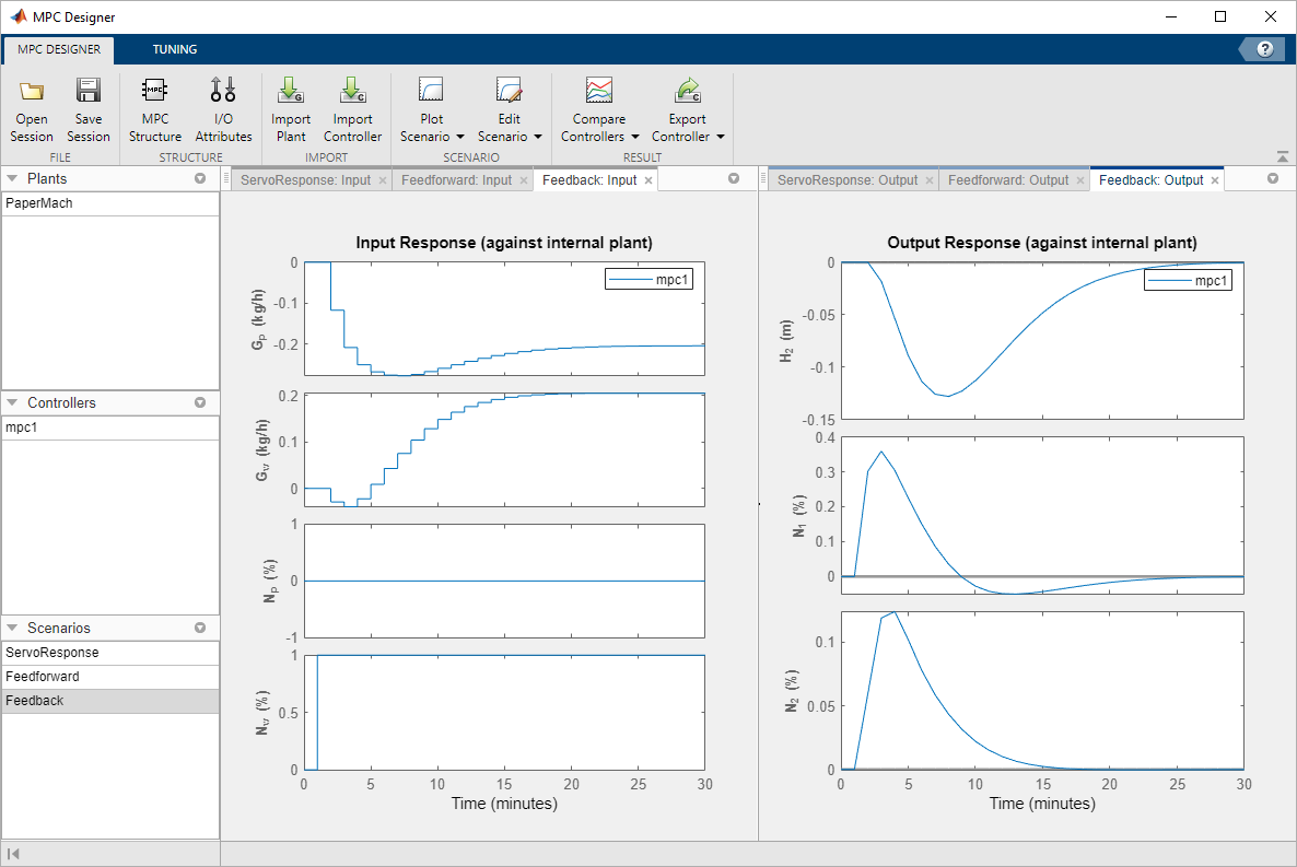
The controlled outputs, H2 and N2, both exhibit relatively small deviations from their setpoints. The settling time is longer than for the original servo response, which is typical.
On the Tuning tab, in the Analysis section, click Review Design to check the controller for potential run-time stability or numerical problems.
The review report opens in a new web browser window.

The review flags two warnings about the controller design. Click the warning names to determine whether they indicate problems with the controller design.
The Closed-Loop Steady-State Gains warning indicates that the plant has more controlled outputs than manipulated variables. This input/output imbalance means that the controller cannot eliminate steady-state error for all of the outputs simultaneously. To meet the control objective of tracking the setpoints of H2 and N2, you previously set the output weight for N1 to zero. This setting causes the QP Hessian Matrix Validity warning, which indicates that one of the output weights is zero.
Because the input/output imbalance is a known feature of the paper machine plant model, and you intentionally set one of the output weights to zero to correct for the imbalance, neither warning indicates an issue with the controller design.
Export Controller to MATLAB Workspace
On the MPC Designer tab, in the Analysis
section, click Export Controller
![]() to save the tuned controller,
to save the tuned controller, mpc1, to
the MATLAB workspace.
Open and Simulate Simulink Model
If you have a Simulink model of your system, you can simulate your controller and validate its performance.
Open the model.
open_system('mpc_papermachine')
The MPC Controller block controls the nonlinear paper machine plant
model, which is defined using the S-Function mpc_pmmodel.
The model is configured to simulate a sustained unmeasured disturbance of size
1.
Double-click the MPC Controller block.
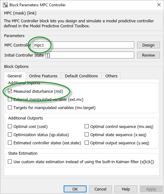
The MPC Controller block is already configured to use the
mpc1 controller that was previously exported to the MATLAB workspace.
Also, the Measured disturbance option is selected to add the
md inport to the controller block.
Simulate the model.
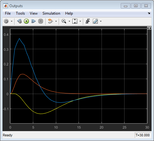
In the Outputs plot, the responses are almost identical to the responses from the corresponding simulation in MPC Designer. The yellow curve is H2, the blue is N1, and the red is N2.
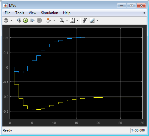
Similarly, in the MVs scope, the manipulated variable moves are almost identical to the moves from corresponding simulation in MPC Designer. The yellow curve is Gp and the blue is Gw.
These results show that there are no significant prediction errors due to the mismatch between the linear prediction model of the controller and the nonlinear plant. Even increasing the unmeasured disturbance magnitude by a factor of four produces similarly shaped response curves. However, as the disturbance size increases further, the effects of nonlinearities become more pronounced.
Increase Unmeasured Disturbance Magnitude
In the Simulink model window, double-click the Unmeasured Disturbance block.
In the Unmeasured Disturbance properties dialog box, specify a Constant
value of 5.5.
Click OK.
Simulate the model.
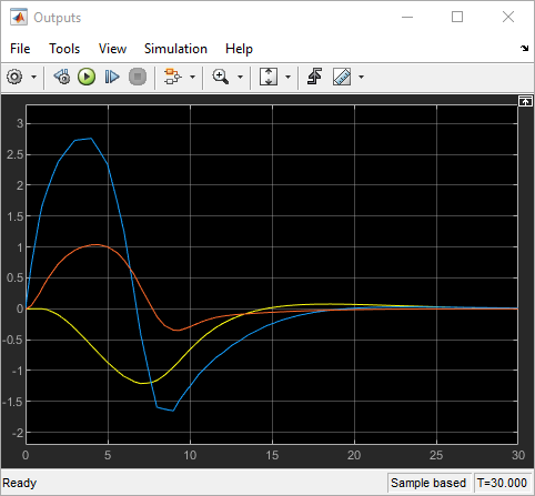
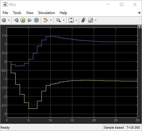
The mismatch between the prediction model and the plant now produces output responses with significant differences. Increasing the disturbance magnitude further results in large setpoint deviations and saturated manipulated variables.
References
[1] Ying, Y., M. Rao, and Y. Sun "Bilinear control strategy for paper making process," Chemical Engineering Communications (1992), Vol. 111, pp. 13–28.