Main Content

ode45

Solve nonstiff differential equations — medium order method

Description

example

[t,y] = ode45(odefun,tspan,y0), where tspan = [t0 tf], integrates the system of differential equations y'=f(t,y) from t0 to tf with initial conditions y0. Each row in the solution array y corresponds to a value returned in column vector t.

All MATLAB® ODE solvers can solve systems of equations of the form y'=f(t,y), or problems that involve a mass matrix, M(t,y)y'=f(t,y). The solvers all use similar syntaxes. The ode23s solver only can solve problems with a mass matrix if the mass matrix is constant. ode15s and ode23t can solve problems with a mass matrix that is singular, known as differential-algebraic equations (DAEs). Specify the mass matrix using the Mass option of odeset.

ode45 is a versatile ODE solver and is the first solver you should try for most problems. However, if the problem is stiff or requires high accuracy, then there are other ODE solvers that might be better suited to the problem. See Choose an ODE Solver for more information.

example

[t,y] = ode45(odefun,tspan,y0,options) also uses the integration settings defined by options, which is an argument created using the odeset function. For example, use the AbsTol and RelTol options to specify absolute and relative error tolerances, or the Mass option to provide a mass matrix.

[t,y,te,ye,ie] = ode45(odefun,tspan,y0,options) additionally finds where functions of (t,y), called event functions, are zero. In the output, te is the time of the event, ye is the solution at the time of the event, and ie is the index of the triggered event.

For each event function, specify whether the integration is to terminate at a zero and whether the direction of the zero crossing matters. Do this by setting the 'Events' property to a function, such as myEventFcn or @myEventFcn, and creating a corresponding function: [value,isterminal,direction] = myEventFcn(t,y). For more information, see ODE Event Location.

example

sol = ode45(___) returns a structure that you can use with deval to evaluate the solution at any point on the interval [t0 tf]. You can use any of the input argument combinations in previous syntaxes.

Examples

collapse all

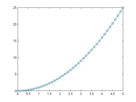
Simple ODEs that have a single solution component can be specified as an anonymous function in the call to the solver. The anonymous function must accept two inputs (t,y), even if one of the inputs is not used in the function.

Solve the ODE

y=2t.

Specify a time interval of [0 5] and the initial condition y0 = 0.

tspan = [0 5];
y0 = 0;
[t,y] = ode45(@(t,y) 2*t, tspan, y0);

Plot the solution.

plot(t,y,'-o')

The van der Pol equation is a second-order ODE

y1-μ(1-y12)y1+y1=0,

where μ>0 is a scalar parameter. Rewrite this equation as a system of first-order ODEs by making the substitution y1=y2. The resulting system of first-order ODEs is

y1=y2y2=μ(1-y12)y2-y1.

The function file vdp1.m represents the van der Pol equation using μ=1. The variables y1 and y2 are the entries y(1) and y(2) of a two-element vector dydt.

function dydt = vdp1(t,y)
%VDP1  Evaluate the van der Pol ODEs for mu = 1
%
%   See also ODE113, ODE23, ODE45.

%   Jacek Kierzenka and Lawrence F. Shampine
%   Copyright 1984-2014 The MathWorks, Inc.

dydt = [y(2); (1-y(1)^2)*y(2)-y(1)];

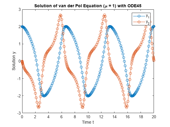
Solve the ODE using the ode45 function on the time interval [0 20] with initial values [2 0]. The resulting output is a column vector of time points t and a solution array y. Each row in y corresponds to a time returned in the corresponding row of t. The first column of y corresponds to y1, and the second column corresponds to y2.

[t,y] = ode45(@vdp1,[0 20],[2; 0]);

Plot the solutions for y1 and y2 against t.

plot(t,y(:,1),'-o',t,y(:,2),'-o')
title('Solution of van der Pol Equation (\mu = 1) with ODE45');
xlabel('Time t');
ylabel('Solution y');
legend('y_1','y_2')

ode45 works only with functions that use two input arguments, t and y. However, you can pass extra parameters by defining them outside the function and passing them in when you specify the function handle.

Solve the ODE

y=ABty.

Rewriting the equation as a first-order system yields

y1=y2y2=ABty1.

odefcn, a local function included at the end of this example, represents this system of equations as a function that accepts four input arguments: t, y, A, and B.

function dydt = odefcn(t,y,A,B)
  dydt = zeros(2,1);
  dydt(1) = y(2);
  dydt(2) = (A/B)*t.*y(1);
end

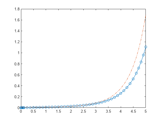
Solve the ODE using ode45. Specify the function handle so that it passes the predefined values for A and B to odefcn.

A = 1;
B = 2;
tspan = [0 5];
y0 = [0 0.01];
[t,y] = ode45(@(t,y) odefcn(t,y,A,B), tspan, y0);

Plot the results.

plot(t,y(:,1),'-o',t,y(:,2),'-.')

function dydt = odefcn(t,y,A,B)
  dydt = zeros(2,1);
  dydt(1) = y(2);
  dydt(2) = (A/B)*t.*y(1);
end

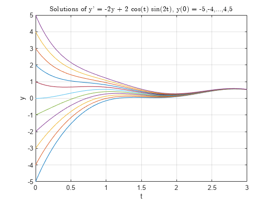
For simple ODE systems with one equation, you can specify y0 as a vector containing multiple initial conditions. This technique creates a system of independent equations through scalar expansion, one for each initial value, and ode45 solves the system to produce results for each initial value.

Create an anonymous function to represent the equation f(t,y)=-2y+2cos(t)sin(2t). The function must accept two inputs for t and y.

yprime = @(t,y) -2*y + 2*cos(t).*sin(2*t);

Create a vector of different initial conditions in the range [-5,5].

y0 = -5:5; 

Solve the equation for each initial condition over the time interval [0,3] using ode45.

tspan = [0 3];
[t,y] = ode45(yprime,tspan,y0);

Plot the results.

plot(t,y)
grid on
xlabel('t')
ylabel('y')
title('Solutions of y'' = -2y + 2 cos(t) sin(2t), y(0) = -5,-4,...,4,5','interpreter','latex')

This technique is useful for solving simple ODEs with several initial conditions. However, the technique also has some tradeoffs:

  • You cannot solve systems of equations with multiple initial conditions. The technique only works when solving one equation with multiple initial conditions.

  • The time step chosen by the solver at each step is based on the equation in the system that needs to take the smallest step. This means the solver can take small steps to satisfy the equation for one initial condition, but the other equations, if solved on their own, would use different step sizes. Despite this, solving for multiple initial conditions at the same time is generally faster than solving the equations separately using a for-loop.

For more information on this technique, see Solve System of ODEs with Multiple Initial Conditions.

Consider the following ODE with time-dependent parameters

$$y'(t) + f(t)y(t) = g(t).$$

The initial condition is $y_0 = 1$. The function f(t) is defined by the n-by-1 vector f evaluated at times ft. The function g(t) is defined by the m-by-1 vector g evaluated at times gt.

Create the vectors f and g.

ft = linspace(0,5,25);
f = ft.^2 - ft - 3;

gt = linspace(1,6,25);
g = 3*sin(gt-0.25);

Write a function named myode that interpolates f and g to obtain the value of the time-dependent terms at the specified time. Save the function in your current folder to run the rest of the example.

The myode function accepts extra input arguments to evaluate the ODE at each time step, but ode45 only uses the first two input arguments t and y.

function dydt = myode(t,y,ft,f,gt,g)
f = interp1(ft,f,t); % Interpolate the data set (ft,f) at time t
g = interp1(gt,g,t); % Interpolate the data set (gt,g) at time t
dydt = -f.*y + g; % Evaluate ODE at time t

Solve the equation over the time interval [1 5] using ode45. Specify the function using a function handle so that ode45 uses only the first two input arguments of myode. Also, loosen the error thresholds using odeset.

tspan = [1 5];
ic = 1;
opts = odeset('RelTol',1e-2,'AbsTol',1e-4);
[t,y] = ode45(@(t,y) myode(t,y,ft,f,gt,g), tspan, ic, opts);

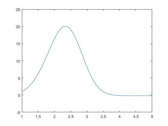
Plot the solution, y, as a function of the time points, t.

plot(t,y)

The van der Pol equation is a second order ODE

y1-μ(1-y12)y1+y1=0.

Solve the van der Pol equation with μ=1 using ode45. The function vdp1.m ships with MATLAB® and encodes the equations. Specify a single output to return a structure containing information about the solution, such as the solver and evaluation points.

tspan = [0 20];
y0 = [2 0];
sol = ode45(@vdp1,tspan,y0)
sol = struct with fields:
     solver: 'ode45'
    extdata: [1x1 struct]
          x: [0 1.0048e-04 6.0285e-04 0.0031 0.0157 0.0785 0.2844 0.5407 0.8788 1.4032 1.8905 2.3778 2.7795 3.1285 3.4093 3.6657 3.9275 4.2944 4.9013 5.3506 5.7998 6.2075 6.5387 6.7519 6.9652 7.2247 7.5719 8.1226 8.6122 9.1017 9.5054 ... ] (1x60 double)
          y: [2x60 double]
      stats: [1x1 struct]
      idata: [1x1 struct]

Use linspace to generate 250 points in the interval [0 20]. Evaluate the solution at these points using deval.

x = linspace(0,20,250);
y = deval(sol,x);

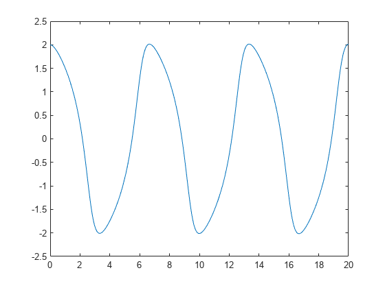
Plot the first component of the solution.

plot(x,y(1,:))

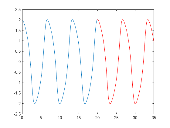
Extend the solution to tf=35 using odextend and add the result to the original plot.

sol_new = odextend(sol,@vdp1,35);
x = linspace(20,35,350);
y = deval(sol_new,x);
hold on
plot(x,y(1,:),'r')

Input Arguments

collapse all

Functions to solve, specified as a function handle that defines the functions to be integrated.

The function dydt = odefun(t,y), for a scalar t and a column vector y, must return a column vector dydt of data type single or double that corresponds to f(t,y). odefun must accept both input arguments t and y, even if one of the arguments is not used in the function.

For example, to solve y'=5y3, use the function:

function dydt = odefun(t,y)
dydt = 5*y-3;
end

For a system of equations, the output of odefun is a vector. Each element in the vector is the computed value of the right side of one equation. For example, consider the system of two equations

y'1=y1+2y2y'2=3y1+2y2

A function that calculates the value of the right side of each equation at each time step is

function dydt = odefun(t,y)
dydt = zeros(2,1);
dydt(1) = y(1)+2*y(2);
dydt(2) = 3*y(1)+2*y(2);
end

For information on how to provide additional parameters to the function odefun, see Parameterizing Functions.

Example: @myFcn

Data Types: function_handle

Interval of integration, specified as a vector. At a minimum, tspan must be a two-element vector [t0 tf] specifying the initial and final times. To obtain solutions at specific times between t0 and tf, use a longer vector of the form [t0,t1,t2,...,tf]. The elements in tspan must be all increasing or all decreasing.

The solver imposes the initial conditions given by y0 at the initial time tspan(1), and then integrates from tspan(1) to tspan(end):

  • If tspan has two elements [t0 tf], then the solver returns the solution evaluated at each internal integration step within the interval.

  • If tspan has more than two elements [t0,t1,t2,...,tf], then the solver returns the solution evaluated at the given points. However, the solver does not step precisely to each point specified in tspan. Instead, the solver uses its own internal steps to compute the solution, and then evaluates the solution at the requested points in tspan. The solutions produced at the specified points are of the same order of accuracy as the solutions computed at each internal step.

    Specifying several intermediate points has little effect on the efficiency of computation, but can affect memory management for large systems.

The values of tspan are used by the solver to calculate suitable values for InitialStep and MaxStep:

  • If tspan contains several intermediate points [t0,t1,t2,...,tf], then the specified points give an indication of the scale for the problem, which can affect the value of InitialStep used by the solver. Therefore, the solution obtained by the solver might be different depending on whether you specify tspan as a two-element vector or as a vector with intermediate points.

  • The initial and final values in tspan are used to calculate the maximum step size MaxStep. Therefore, changing the initial or final values in tspan can cause the solver to use a different step sequence, which might change the solution.

Example: [1 10]

Example: [1 3 5 7 9 10]

Data Types: single | double

Initial conditions, specified as a vector. y0 must be the same length as the vector output of odefun, so that y0 contains an initial condition for each equation defined in odefun.

Data Types: single | double

Option structure, specified as a structure array. Use the odeset function to create or modify the options structure. See Summary of ODE Options for a list of the options compatible with each solver.

Example: options = odeset('RelTol',1e-5,'Stats','on','OutputFcn',@odeplot) specifies a relative error tolerance of 1e-5, turns on the display of solver statistics, and specifies the output function @odeplot to plot the solution as it is computed.

Data Types: struct

Output Arguments

collapse all

Evaluation points, returned as a column vector.

  • If tspan contains two elements [t0 tf], then t contains the internal evaluation points used to perform the integration.

  • If tspan contains more than two elements, then t is the same as tspan.

Solutions, returned as an array. Each row in y corresponds to the solution at the value returned in the corresponding row of t.

Time of events, returned as a column vector. The event times in te correspond to the solutions returned in ye, and ie specifies which event occurred.

Solution at time of events, returned as an array. The event times in te correspond to the solutions returned in ye, and ie specifies which event occurred.

Index of triggered event function, returned as a column vector. The event times in te correspond to the solutions returned in ye, and ie specifies which event occurred.

Structure for evaluation, returned as a structure array. Use this structure with the deval function to evaluate the solution at any point in the interval [t0 tf]. The sol structure array always includes these fields:

Structure FieldDescription

sol.x

Row vector of the steps chosen by the solver.

sol.y

Solutions. Each column sol.y(:,i) contains the solution at time sol.x(i).

sol.solver

Solver name.

Additionally, if you specify the Events option of odeset and events are detected, then sol also includes these fields:

Structure FieldDescription

sol.xe

Points when events occurred. sol.xe(end) contains the exact point of a terminal event, if any.

sol.ye

Solutions that correspond to events in sol.xe.

sol.ie

Indices into the vector returned by the function specified in the Events option. The values indicate which event the solver detected.

Algorithms

ode45 is based on an explicit Runge-Kutta (4,5) formula, the Dormand-Prince pair. It is a single-step solver – in computing y(tn), it needs only the solution at the immediately preceding time point, y(tn-1) [1], [2].

References

[1] Dormand, J. R. and P. J. Prince, “A family of embedded Runge-Kutta formulae,” J. Comp. Appl. Math., Vol. 6, 1980, pp. 19–26.

[2] Shampine, L. F. and M. W. Reichelt, “The MATLAB ODE Suite,” SIAM Journal on Scientific Computing, Vol. 18, 1997, pp. 1–22.

Extended Capabilities

Version History

Introduced before R2006a