Main Content

ode15s

Solve stiff differential equations and DAEs — variable order method

Description

example

[t,y] = ode15s(odefun,tspan,y0), where tspan = [t0 tf], integrates the system of differential equations y'=f(t,y) from t0 to tf with initial conditions y0. Each row in the solution array y corresponds to a value returned in column vector t.

All MATLAB® ODE solvers can solve systems of equations of the form y'=f(t,y), or problems that involve a mass matrix, M(t,y)y'=f(t,y). The solvers all use similar syntaxes. The ode23s solver only can solve problems with a mass matrix if the mass matrix is constant. ode15s and ode23t can solve problems with a mass matrix that is singular, known as differential-algebraic equations (DAEs). Specify the mass matrix using the Mass option of odeset.

example

[t,y] = ode15s(odefun,tspan,y0,options) also uses the integration settings defined by options, which is an argument created using the odeset function. For example, use the AbsTol and RelTol options to specify absolute and relative error tolerances, or the Mass option to provide a mass matrix.

[t,y,te,ye,ie] = ode15s(odefun,tspan,y0,options) additionally finds where functions of (t,y), called event functions, are zero. In the output, te is the time of the event, ye is the solution at the time of the event, and ie is the index of the triggered event.

For each event function, specify whether the integration is to terminate at a zero and whether the direction of the zero crossing matters. Do this by setting the 'Events' property to a function, such as myEventFcn or @myEventFcn, and creating a corresponding function: [value,isterminal,direction] = myEventFcn(t,y). For more information, see ODE Event Location.

example

sol = ode15s(___) returns a structure that you can use with deval to evaluate the solution at any point on the interval [t0 tf]. You can use any of the input argument combinations in previous syntaxes.

Examples

collapse all

Simple ODEs that have a single solution component can be specified as an anonymous function in the call to the solver. The anonymous function must accept two inputs (t,y), even if one of the inputs is not used in the function.

Solve the ODE

y=-10t.

Specify a time interval of [0 2] and the initial condition y0 = 1.

tspan = [0 2];
y0 = 1;
[t,y] = ode15s(@(t,y) -10*t, tspan, y0);

Plot the solution.

plot(t,y,'-o')

An example of a stiff system of equations is the van der Pol equations in relaxation oscillation. The limit cycle has regions where the solution components change slowly and the problem is quite stiff, alternating with regions of very sharp change where it is not stiff.

The system of equations is:

$$\begin{array}{cl} y_1' &= y_2\\y_2' &= 1000(1-y_1^2)y_2-y_1\end{array}$$

The initial conditions are $y_1(0)=2$ and $y_2(0)=0$. The function vdp1000 ships with MATLAB® and encodes the equations.

function dydt = vdp1000(t,y)
%VDP1000  Evaluate the van der Pol ODEs for mu = 1000.
%
%   See also ODE15S, ODE23S, ODE23T, ODE23TB.

%   Jacek Kierzenka and Lawrence F. Shampine
%   Copyright 1984-2014 The MathWorks, Inc.

dydt = [y(2); 1000*(1-y(1)^2)*y(2)-y(1)];

Solving this system using ode45 with the default relative and absolute error tolerances (1e-3 and 1e-6, respectively) is extremely slow, requiring several minutes to solve and plot the solution. ode45 requires millions of time steps to complete the integration, due to the areas of stiffness where it struggles to meet the tolerances.

This is a plot of the solution obtained by ode45, which takes a long time to compute. Notice the enormous number of time steps required to pass through areas of stiffness.

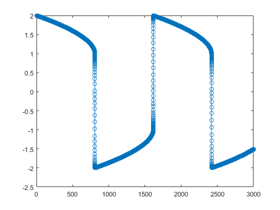
Solve the stiff system using the ode15s solver, and then plot the first column of the solution y against the time points t. The ode15s solver passes through stiff areas with far fewer steps than ode45.

[t,y] = ode15s(@vdp1000,[0 3000],[2 0]);
plot(t,y(:,1),'-o')

ode15s only works with functions that use two input arguments, t and y. However, you can pass in extra parameters by defining them outside the function and passing them in when you specify the function handle.

Solve the ODE

$$y'' = \frac{A}{B} t y.$$

Rewriting the equation as a first-order system yields

$$\begin{array}{cl} y'_1 &= y_2\\ y'_2 &= \frac{A}{B} t y_1.
\end{array}$$

odefcn.m represents this system of equations as a function that accepts four input arguments: t, y, A, and B.

function dydt = odefcn(t,y,A,B)
dydt = zeros(2,1);
dydt(1) = y(2);
dydt(2) = (A/B)*t.*y(1);

Solve the ODE using ode15s. Specify the function handle such that it passes in the predefined values for A and B to odefcn.

A = 1;
B = 2;
tspan = [0 5];
y0 = [0 0.01];
[t,y] = ode15s(@(t,y) odefcn(t,y,A,B), tspan, y0);

Plot the results.

plot(t,y(:,1),'-o',t,y(:,2),'-.')

The ode15s solver is a good first choice for most stiff problems. However, the other stiff solvers might be more efficient for certain types of problems. This example solves a stiff test equation using all four stiff ODE solvers.

Consider the test equation

y=-λy.

The equation becomes increasingly stiff as the magnitude of λ increases. Use λ=1×10⁹ and the initial condition y(0)=1 over the time interval [0 0.5]. With these values, the problem is stiff enough that ode45 and ode23 struggle to integrate the equation. Also, use odeset to pass in the constant Jacobian J=fy=-λ and turn on the display of solver statistics.

lambda = 1e9;
y0 = 1;
tspan = [0 0.5];
opts = odeset('Jacobian',-lambda,'Stats','on');

Solve the equation with ode15s, ode23s, ode23t, and ode23tb. Make subplots for comparison.

subplot(2,2,1)
tic, ode15s(@(t,y) -lambda*y, tspan, y0, opts), toc
104 successful steps
1 failed attempts
212 function evaluations
0 partial derivatives
21 LU decompositions
210 solutions of linear systems
Elapsed time is 1.117982 seconds.
title('ode15s')
subplot(2,2,2)
tic, ode23s(@(t,y) -lambda*y, tspan, y0, opts), toc
63 successful steps
0 failed attempts
191 function evaluations
0 partial derivatives
63 LU decompositions
189 solutions of linear systems
Elapsed time is 0.179014 seconds.
title('ode23s')
subplot(2,2,3)
tic, ode23t(@(t,y) -lambda*y, tspan, y0, opts), toc
95 successful steps
0 failed attempts
125 function evaluations
0 partial derivatives
28 LU decompositions
123 solutions of linear systems
Elapsed time is 0.233392 seconds.
title('ode23t')
subplot(2,2,4)
tic, ode23tb(@(t,y) -lambda*y, tspan, y0, opts), toc
71 successful steps
0 failed attempts
167 function evaluations
0 partial derivatives
23 LU decompositions
236 solutions of linear systems
Elapsed time is 0.234603 seconds.
title('ode23tb')

The stiff solvers all perform well, but ode23s completes the integration with the fewest steps and runs the fastest for this particular problem. Since the constant Jacobian is specified, none of the solvers need to calculate partial derivatives to compute the solution. Specifying the Jacobian benefits ode23s the most since it normally evaluates the Jacobian in every step.

For general stiff problems, the performance of the stiff solvers varies depending on the format of the problem and specified options. Providing the Jacobian matrix or sparsity pattern always improves solver efficiency for stiff problems. But since the stiff solvers use the Jacobian differently, the improvement can vary significantly. Practically speaking, if a system of equations is very large or needs to be solved many times, then it is worthwhile to investigate the performance of the different solvers to minimize execution time.

The van der Pol equation is a second order ODE

y1-μ(1-y12)y1+y1=0.

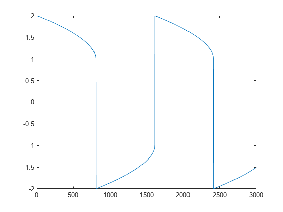
Solve the van der Pol equation with μ=1000 using ode15s. The function vdp1000.m ships with MATLAB® and encodes the equations. Specify a single output to return a structure containing information about the solution, such as the solver and evaluation points.

tspan = [0 3000];
y0 = [2 0];
sol = ode15s(@vdp1000,tspan,y0)
sol = struct with fields:
     solver: 'ode15s'
    extdata: [1x1 struct]
          x: [0 1.4606e-05 2.9212e-05 4.3818e-05 1.1010e-04 1.7639e-04 2.4267e-04 3.0896e-04 4.5006e-04 5.9116e-04 7.3226e-04 8.7336e-04 0.0010 0.0012 0.0013 0.0015 0.0017 0.0018 0.0021 0.0024 0.0027 0.0030 0.0033 0.0044 0.0055 0.0066 ... ] (1x592 double)
          y: [2x592 double]
      stats: [1x1 struct]
      idata: [1x1 struct]

Use linspace to generate 2500 points in the interval [0 3000]. Evaluate the first component of the solution at these points using deval.

x = linspace(0,3000,2500);
y = deval(sol,x,1);

Plot the solution.

plot(x,y)

Extend the solution to tf=4000 using odextend and add the result to the original plot.

tf = 4000;
sol_new = odextend(sol,@vdp1000,tf);
x = linspace(3000,tf,350);
y = deval(sol_new,x,1);
hold on
plot(x,y,'r')

This example reformulates a system of ODEs as a system of differential algebraic equations (DAEs). The Robertson problem found in hb1ode.m is a classic test problem for programs that solve stiff ODEs. The system of equations is

$$\begin{array}{cl} y'_1 &= -0.04y_1 + 10^4 y_2y_3\\ y'_2 &= 0.04y_1 -
10^4 y_2y_3- (3 \times 10^7)y_2^2\\ y'_3 &= (3 \times
10^7)y_2^2.\end{array}$$

hb1ode solves this system of ODEs to steady state with the initial conditions $y_1 = 1$, $y_2 = 0$, and $y_3 = 0$. But the equations also satisfy a linear conservation law,

$$y'_1 + y'_2 + y'_3 = 0.$$

In terms of the solution and initial conditions, the conservation law is

$$y_1 + y_2 + y_3 = 1.$$

The system of equations can be rewritten as a system of DAEs by using the conservation law to determine the state of $y_3$. This reformulates the problem as the DAE system

$$\begin{array}{cl} y'_1 &= -0.04y_1 + 10^4 y_2y_3\\ y'_2 &= 0.04y_1 -
10^4 y_2y_3-(3 \times 10^7)y_2^2\\ 0 &= y_1 + y_2 + y_3 - 1.\end{array}$$

The differential index of this system is 1, since only a single derivative of $y_3$ is required to make this a system of ODEs. Therefore, no further transformations are required before solving the system.

The function robertsdae encodes this DAE system. Save robertsdae.m in your current folder to run the example.

function out = robertsdae(t,y)
out = [-0.04*y(1) + 1e4*y(2).*y(3)
   0.04*y(1) - 1e4*y(2).*y(3) - 3e7*y(2).^2
   y(1) + y(2) + y(3) - 1 ];

The full example code for this formulation of the Robertson problem is available in hb1dae.m.

Solve the DAE system using ode15s. Consistent initial conditions for y0 are obvious based on the conservation law. Use odeset to set the options:

  • Use a constant mass matrix to represent the left hand side of the system of equations.

$$\left( \begin{array}{c} y'_1\\ y'_2\\ 0 \end{array} \right) = M y'
\rightarrow M = \left( \begin{array}{ccc} 1 & 0 & 0\\ 0 & 1 & 0\\ 0 & 0 &
0 \end{array} \right)$$

  • Set the relative error tolerance to 1e-4.

  • Use an absolute tolerance of 1e-10 for the second solution component, since the scale varies dramatically from the other components.

  • Leave the 'MassSingular' option at its default value 'maybe' to test the automatic detection of a DAE.

y0 = [1; 0; 0];
tspan = [0 4*logspace(-6,6)];
M = [1 0 0; 0 1 0; 0 0 0];
options = odeset('Mass',M,'RelTol',1e-4,'AbsTol',[1e-6 1e-10 1e-6]);
[t,y] = ode15s(@robertsdae,tspan,y0,options);

Plot the solution.

y(:,2) = 1e4*y(:,2);
semilogx(t,y);
ylabel('1e4 * y(:,2)');
title('Robertson DAE problem with a Conservation Law, solved by ODE15S');

Input Arguments

collapse all

Functions to solve, specified as a function handle that defines the functions to be integrated.

The function dydt = odefun(t,y), for a scalar t and a column vector y, must return a column vector dydt of data type single or double that corresponds to f(t,y). odefun must accept both input arguments t and y, even if one of the arguments is not used in the function.

For example, to solve y'=5y3, use the function:

function dydt = odefun(t,y)
dydt = 5*y-3;
end

For a system of equations, the output of odefun is a vector. Each element in the vector is the computed value of the right side of one equation. For example, consider the system of two equations

y'1=y1+2y2y'2=3y1+2y2

A function that calculates the value of the right side of each equation at each time step is

function dydt = odefun(t,y)
dydt = zeros(2,1);
dydt(1) = y(1)+2*y(2);
dydt(2) = 3*y(1)+2*y(2);
end

For information on how to provide additional parameters to the function odefun, see Parameterizing Functions.

Example: @myFcn

Data Types: function_handle

Interval of integration, specified as a vector. At a minimum, tspan must be a two-element vector [t0 tf] specifying the initial and final times. To obtain solutions at specific times between t0 and tf, use a longer vector of the form [t0,t1,t2,...,tf]. The elements in tspan must be all increasing or all decreasing.

The solver imposes the initial conditions given by y0 at the initial time tspan(1), and then integrates from tspan(1) to tspan(end):

  • If tspan has two elements [t0 tf], then the solver returns the solution evaluated at each internal integration step within the interval.

  • If tspan has more than two elements [t0,t1,t2,...,tf], then the solver returns the solution evaluated at the given points. However, the solver does not step precisely to each point specified in tspan. Instead, the solver uses its own internal steps to compute the solution, and then evaluates the solution at the requested points in tspan. The solutions produced at the specified points are of the same order of accuracy as the solutions computed at each internal step.

    Specifying several intermediate points has little effect on the efficiency of computation, but can affect memory management for large systems.

The values of tspan are used by the solver to calculate suitable values for InitialStep and MaxStep:

  • If tspan contains several intermediate points [t0,t1,t2,...,tf], then the specified points give an indication of the scale for the problem, which can affect the value of InitialStep used by the solver. Therefore, the solution obtained by the solver might be different depending on whether you specify tspan as a two-element vector or as a vector with intermediate points.

  • The initial and final values in tspan are used to calculate the maximum step size MaxStep. Therefore, changing the initial or final values in tspan can cause the solver to use a different step sequence, which might change the solution.

Example: [1 10]

Example: [1 3 5 7 9 10]

Data Types: single | double

Initial conditions, specified as a vector. y0 must be the same length as the vector output of odefun, so that y0 contains an initial condition for each equation defined in odefun.

Data Types: single | double

Option structure, specified as a structure array. Use the odeset function to create or modify the options structure. See Summary of ODE Options for a list of the options compatible with each solver.

Example: options = odeset('RelTol',1e-5,'Stats','on','OutputFcn',@odeplot) specifies a relative error tolerance of 1e-5, turns on the display of solver statistics, and specifies the output function @odeplot to plot the solution as it is computed.

Data Types: struct

Output Arguments

collapse all

Evaluation points, returned as a column vector.

  • If tspan contains two elements [t0 tf], then t contains the internal evaluation points used to perform the integration.

  • If tspan contains more than two elements, then t is the same as tspan.

Solutions, returned as an array. Each row in y corresponds to the solution at the value returned in the corresponding row of t.

Time of events, returned as a column vector. The event times in te correspond to the solutions returned in ye, and ie specifies which event occurred.

Solution at time of events, returned as an array. The event times in te correspond to the solutions returned in ye, and ie specifies which event occurred.

Index of triggered event function, returned as a column vector. The event times in te correspond to the solutions returned in ye, and ie specifies which event occurred.

Structure for evaluation, returned as a structure array. Use this structure with the deval function to evaluate the solution at any point in the interval [t0 tf]. The sol structure array always includes these fields:

Structure FieldDescription

sol.x

Row vector of the steps chosen by the solver.

sol.y

Solutions. Each column sol.y(:,i) contains the solution at time sol.x(i).

sol.solver

Solver name.

Additionally, if you specify the Events option of odeset and events are detected, then sol also includes these fields:

Structure FieldDescription

sol.xe

Points when events occurred. sol.xe(end) contains the exact point of a terminal event, if any.

sol.ye

Solutions that correspond to events in sol.xe.

sol.ie

Indices into the vector returned by the function specified in the Events option. The values indicate which event the solver detected.

Algorithms

ode15s is a variable-step, variable-order (VSVO) solver based on the numerical differentiation formulas (NDFs) of orders 1 to 5. Optionally, it can use the backward differentiation formulas (BDFs, also known as Gear's method) that are usually less efficient. Like ode113, ode15s is a multistep solver. Use ode15s if ode45 fails or is very inefficient and you suspect that the problem is stiff, or when solving a differential-algebraic equation (DAE) [1], [2].

References

[1] Shampine, L. F. and M. W. Reichelt, “The MATLAB ODE Suite,” SIAM Journal on Scientific Computing, Vol. 18, 1997, pp. 1–22.

[2] Shampine, L. F., M. W. Reichelt, and J.A. Kierzenka, “Solving Index-1 DAEs in MATLAB and Simulink,” SIAM Review, Vol. 41, 1999, pp. 538–552.

Extended Capabilities

Version History

Introduced before R2006a