Find and Remove Trends

Find and remove polynomial or periodic trends from data in the Live Editor

Description

The Find and Remove Trends task lets you interactively identify polynomial or periodic trends in data and return or remove them. The task automatically generates MATLAB^® code for your live script. For more information about Live Editor tasks generally, see Add Interactive Tasks to a Live Script.

Using this task, you can:

• Identify a polynomial trend in data.

  • Choose the degree of the polynomial trend to remove from data.

  • Dynamically arrange breakpoints to define piecewise segments of the data.

  • Specify continuity constraints.

  • Visualize and return the computed trends and data with the trends removed.

• Identify long-term and periodic, seasonal, or oscillatory trends in data.

  • Choose the Singular Spectrum Analysis (SSA) or Seasonal Trend Decomposition Using Loess (STL) algorithm to find trends in the data.

  • Specify the number of periodic trends and lag window when the periods of trends are unknown.

  • Specify period lengths when the periods of trends are known.

  • Visualize and return the computed trends and data with the trends removed.

More

Related Functions

Find and Remove Trends generates code that uses the detrend and trenddecomp functions.

×

Open the Task

To add the Find and Remove Trends task to a live script in the MATLAB Editor:

• On the Live Editor tab, select Task > Find and Remove Trends.

• In a code block in the script, type a relevant keyword, such as find, remove, detrend, trenddecomp, stl, or ssa. Select Find and Remove Trends from the suggested command completions. Then, select the trend type. For some keywords, the task automatically updates one or more corresponding parameters.

Examples

Remove Linear Polynomial Trend

Interactively identify and remove a linear trend in array data with the Find and Remove Trends task in the Live Editor.

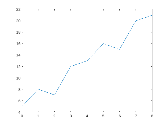
Create a vector x containing some fluctuation. Create a plot to visualize the data.

t = 0:8;
trend = 2*t+5;
sig = [0 1 -2 1 0 1 -2 1 0];
data = sig + trend;
plot(t,data)

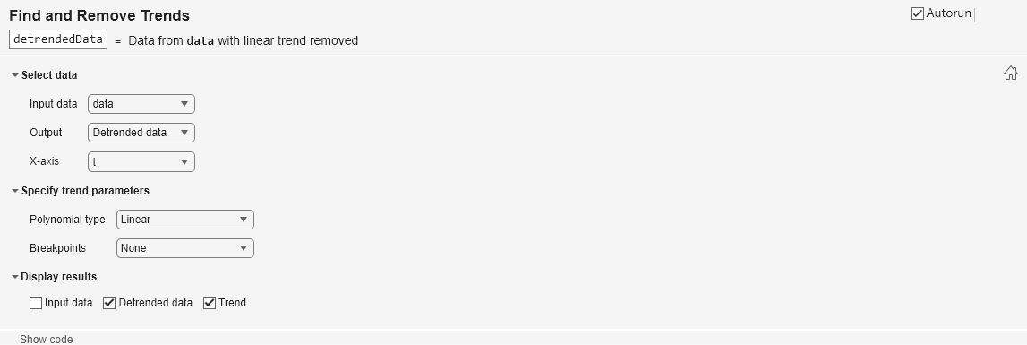
Add the Find and Remove Trends task to the live script. Because the data has a polynomial trend, choose the Polynomial trend type.

Remove the polynomial trend from the data. Select data as the input data and Detrended data as the output to return. Alternatively, you can use the Output field to return the trend. Select t as the x-axis values associated with the input data. Identify a linear trend by specifying the polynomial type as Linear.

Display the resulting trend and the detrended data in a stacked plot.

Remove Piecewise Polynomial Trend

Interactively identify and remove a piecewise polynomial trend in array data using the Find and Remove Trends task in the Live Editor.

A polynomial trend is a trend that best describes fluctuating data. A polynomial trend is used when your data both increases and decreases in value, and the degree of the polynomial trend increases as the data fluctuates.

Consider an electrocardiogram (ECG) signal that shows a pattern not intrinsic to the data that must be removed. Load the signal ecgnl using the sample file ecgSignals.mat and plot the signal.

load("ecgSignals.mat","ecgnl")

plot(ecgnl)
title("ECG Signals with Trends")
xlabel("Sample")
ylabel("Voltage (mV)")

Then, eliminate the nonlinear trend. Add the Find and Remove Trends task to the live script. Because the data has a polynomial trend, choose the Polynomial trend type.

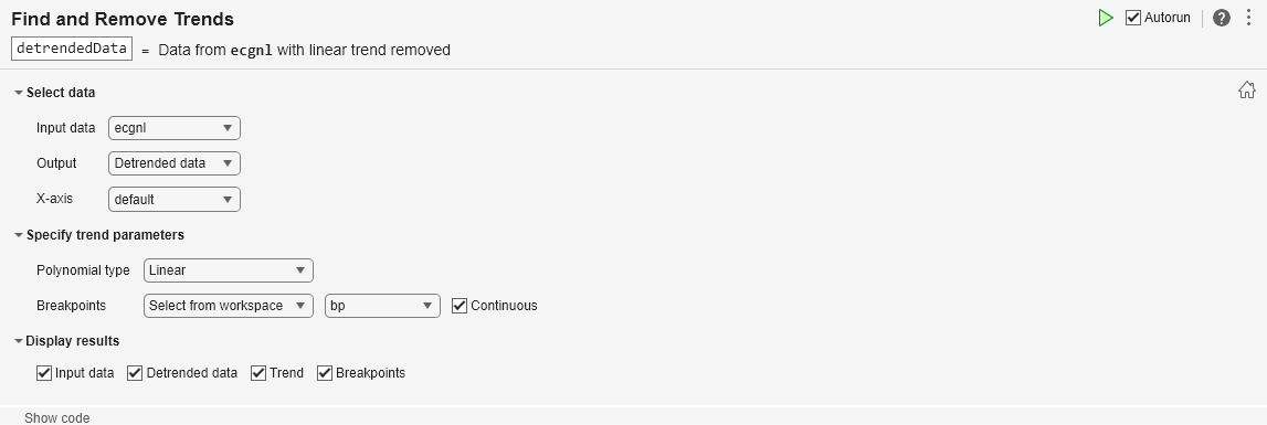
Operate on the signal by selecting ecgnl as the input data. Select Detrended data as the output. The default x-axis values are the sample numbers. Because the wander of the heart rhythm does not occur with consistent frequency, identify a piecewise trend by specifying a vector of breakpoints in the sample data. Alternatively, you can select the breakpoints from a plot.

bp = [160 660 1160 1660];

Then, choose a custom polynomial type and specify the polynomial degree as 5. The resulting visualization displays the input data, piecewise polynomial trend, and the data with the trend removed. The detrended data is returned in detrendedData and has the same size as ecgnl. Alternatively, to return the trend, use the Output field.

Find Periodic Trends Using STL

Interactively decompose array data into its long-term trend, two periodic trends, and remainder using the seasonal trend decomposition using loess (STL) algorithm with the Find and Remove Trends task in the Live Editor.

Create a variable data that contains a long-term trend, two seasonal trends with different periods, and a noise component. Create a plot to visualize the data.

t = (1:200)';
trend = 0.001*(t-100).^2;
period1 = 20;
period2 = 30;
seasonal1 = 2*sin(2*pi*t/period1);
seasonal2 = 0.75*sin(2*pi*t/period2);
noise = 2*(rand(200,1) - 0.5);
data = trend + seasonal1 + seasonal2 + noise;

plot(data)

Add the Find and Remove Trends task to the live script. Because the data has a recurring, periodic trend, choose the Periodic trend type.

Decompose the data into its trend components by selecting data as the input data and All trends as the output to return. Because the periods of the seasonal trends in the data are known, choose the STL algorithm and specify the known period lengths as 20 and 30 data points.

Display the input data and the resulting long-term trend, two periodic trends, and remainder in a stacked plot. The Live Editor task returns the identified trends in arrays longterm and periodic. Alternatively, to return the detrended data, use the Output field to specify which trend types to remove.

Resample Irregular Data and Find Periodic Trends Using SSA

Interactively identify and return periodic trends using the singular spectrum analysis (SSA) algorithm with the Find and Remove Trends task in the Live Editor.

Consider a timetable of monthly international airline passenger totals from 1949 to 1960. Load the timetable using the sample file Data_Airline.mat and plot the passenger data.

load("Data_Airline.mat","DataTimeTable");

plot(DataTimeTable,"Time","PSSG")
title("Passenger Data")

Notice that the timetable is irregularly spaced. The Find and Remove Trends task requires that the input timetable is regularly spaced.

isregular(DataTimeTable.Time)

ans = logical
   0

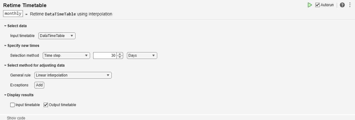
Make the timetable regular by resampling using the Retime Timetable task in the Live Editor. Interpolate the data onto a regular time vector with a time step of 30 days and return the resampled data in a timetable named monthly.

monthly=147×1 timetable
       Time         PSSG 
    ___________    ______

    01-Jan-1949       112
    31-Jan-1949    117.81
    02-Mar-1949     131.9
    01-Apr-1949       129
    01-May-1949       121
    31-May-1949    134.55
    30-Jun-1949    147.57
    30-Jul-1949       148
    29-Aug-1949    137.16
    28-Sep-1949     120.7
    28-Oct-1949    105.94
    27-Nov-1949    116.13
    27-Dec-1949    115.48
    26-Jan-1950    123.87
    25-Feb-1950    138.86
    27-Mar-1950    135.97
      ⋮

isregular(monthly.Time)

ans = logical
   1

The airline passenger data shows an increase in the seasonal variance over time. Because the Find and Remove Trends task analyzes the series using additive decomposition models, apply a log transformation to the data.

monthly.PSSGLog = log(monthly.PSSG);

Then, identify periodic trends in the passenger data by adding the Find and Remove Trends task to the live script. Because the data has a recurring, periodic trend, choose the Periodic trend type.

Operate on the passenger totals by specifying the input data as the PSSGLog variable of monthly. Because the periods of the seasonal trends in the data are unknown, choose the SSA algorithm. Increase the number of periodic trends until the baseline of the remainder is flat.

Display the input data and the resulting long-term trend, four periodic trends, and remainder in a stacked plot. The Live Editor task returns the identified trends in the array trends. Alternatively, to return the detrended data, use the Output field to specify which trend types to remove.

Related Examples

• Add Interactive Tasks to a Live Script
• Clean Messy Data and Locate Extrema Using Live Editor Tasks

Parameters

Polynomial Trends

Input data — Valid input data from workspace

vector | matrix | multidimensional array | table | timetable

This task operates on input data contained in a vector, matrix, multidimensional array, table, or timetable. The data can be of type single or double.

For table or timetable input data, this task operates on each table variable separately. To operate on all variables with type single or double, select All supported variables. To choose which single or double variables to operate on, select Specified variables.

Periodic Trends

Input data — Valid input data from workspace

vector | table | timetable

This task operates on input data contained in a vector, table, or timetable. The data can be of type single or double. For timetable input data, the vector of row times must be regularly spaced.

For table or timetable input data, this task operates on each table variable separately. To operate on all variables with type single or double, select All supported variables. To choose which single or double variables to operate on, select Specified variables.

Tips

• If your data has seasonal variation that is proportional to the level of the time series, use a log transformation on the data before looking for periodic trends.

Algorithms

Breakpoints

For a polynomial trend, use the Breakpoints field to specify the location of breakpoints. A breakpoint is a point in the range of x that separates intervals and identifies a piecewise trend consisting of multiple subfunctions. A piecewise trend can be continuous, where the limits of subfunctions as they approach a breakpoint are equal, or discontinuous, where the limits are not equal.

Singular Spectrum Analysis (SSA)

For a periodic trend, use the Algorithm field to specify SSA. SSA is an additive decomposition model used for regularly spaced time series when the periods of recurring, periodic trends are unknown. The algorithm uses singular value decomposition (SVD) to decompose a time series into a specified number of periodic trends. A lag value determines the size of the matrix on which the SVD is computed. Larger lag window values typically result in more separation of the trends.

An additive decomposition model decomposes time series data such that A = LT+ST+R, where LT is the long-term trend in the data, ST is the seasonal, or oscillatory, trend (or trends), and R is the remainder.

Seasonal Trend Decomposition Using Loess (STL)

For a periodic trend, use the Algorithm field to specify STL. STL is an additive decomposition model used for regularly spaced time series when the periods of recurring, periodic trends are known. The algorithm uses loess (locally weighted smoothing) to decompose a time series into periods of specified lengths.

An additive decomposition model decomposes time series data such that A = LT+ST+R, where LT is the long-term trend in the data, ST is the seasonal, or oscillatory, trend (or trends), and R is the remainder.

Version History

Introduced in R2019b

R2023a: Find and remove periodic and polynomial trends

In addition to identifying polynomial trends, you can now interactively identify periodic trends for regularly spaced input data. Select the trend type as Periodic, and choose the SSA or STL algorithm.

You can also return polynomial and periodic trend data, in addition to the detrended data, using this Live Editor task. Specify the Output as Trends.

Previously, this task identified only polynomial trends and returned only the detrended data.

R2023a: Renamed from Remove Trends

To reflect the enhanced functionality, this task is now named Find and Remove Trends. Previously, this task was named Remove Trends.

R2022b: Plot multiple table variables

Simultaneously plot multiple table variables in the display of this Live Editor task. For table or timetable data, to visualize all selected table variables at once in a tiled chart layout, set the Variable to display field.

R2022b: Append detrended table variables

Append input table variables with table variables containing detrended data. For table or timetable input data, to append the detrended data, set the Output format field.

R2022a: Live Editor task does not run automatically if input is large

This Live Editor task does not run automatically if the input data is large. In previous releases, the task always ran automatically for inputs of any size. If the inputs have a large number of elements, then the code generated by this task can take a noticeable amount of time to run (more than a few seconds).

When a task does not run automatically, the Autorun indicator is disabled. You can either run the task manually when needed or choose to enable the task to run automatically.

R2021a: Operate on multiple table variables

This Live Editor task can operate on multiple table variables at the same time. For table or timetable input data, to operate on multiple variables, select All supported variables or Specified variables. Return all of the variables or only the modified variables, and specify which variable to visualize.