Solve Equations of Motion for Baton Thrown into Air
This example solves a system of ordinary differential equations that model the dynamics of a baton thrown into the air [1]. The baton is modeled as two particles with masses and connected by a rod of length . The baton is thrown into the air and subsequently moves in the vertical xy-plane subject to the force due to gravity. The rod forms an angle with the horizontal and the coordinates of the first mass are . With this formulation, the coordinates of the second mass are .
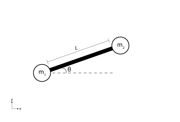
The equations of motion for the system are obtained by applying Lagrange's equations for each of the three coordinates, , , and :
Code Equations
MATLAB requires the equations to be written in the form , where is the first derivative of each coordinate. In this problem, the solution vector has six components: , , the angle , and their first derivatives:
With this notation, you can rewrite the equations of motion entirely in terms of the elements of :
Unfortunately, the equations of motion do not fit into the form required by the solver, since there are several terms on the left with first derivatives. When this occurs, you must use a mass matrix to represent the left side of the equation.
With matrix notation, you can rewrite the equations of motion as a system of six equations using a mass matrix in the form . The mass matrix expresses the linear combinations of first derivatives on the left side of the equation with a matrix-vector product. In this form, the system of equations becomes:
From this expression, you can write a function that calculates the nonzero elements of the mass matrix. The function takes three inputs: and the solution vector are required (you must specify these inputs even if they are not used in the body of the function), and is an optional extra input used to pass in parameter values.
function M = mass(t,q,P)
% Extract parameters
m1 = P(1);
m2 = P(2);
L = P(3);
g = P(4);

% Mass matrix elements
M = zeros(6,6);
M(1,1) = 1;
M(2,2) = m1 + m2;
M(2,6) = -m2*L*sin(q(5));
M(3,3) = 1;
M(4,4) = m1 + m2;
M(4,6) = m2*L*cos(q(5));
M(5,5) = 1;
M(6,2) = -L*sin(q(5));
M(6,4) = L*cos(q(5));
M(6,6) = L^2;
end
Next, you can write a function for the right side of each of the equations in the system . Like the mass matrix function, this function takes two required inputs for and , and one optional input for parameter values .
function dydt = f(t,q,P)
% Extract parameters
m1 = P(1);
m2 = P(2);
L = P(3);
g = P(4);

% Equations to solve
dydt = [q(2)
        m2*L*q(6)^2*cos(q(5))
        q(4)
        m2*L*q(6)^2*sin(q(5))-(m1+m2)*g
        q(6)
        -g*L*cos(q(5))];
end
Solve System of Equations
First, create a vector P of parameter values for , , , and . The solver passes the vector P to the mass matrix and ODE functions as an extra input.
P = [0.1 0.1 1 9.81];
Create a vector of initial conditions for the problem. Since the baton is thrown upward at an angle, use nonzero values for the initial velocities, , , and . For the initial positions, the baton begins in an upright position, so , , and .
y0 = [0; 4; P(3); 20; -pi/2; 2];
Now, create an ode object to represent the problem, specifying values for ODEFcn, MassMatrix, InitialValue, and Parameters. The object display indicates that the ode15s solver is chosen for the problem since a mass matrix is present.
F = ode(ODEFcn=@f,...
        MassMatrix=@mass,...
        InitialValue=y0,...
        Parameters=P)
F =
  ode with properties:

   Problem definition
               ODEFcn: @f
           Parameters: [0.1000 0.1000 1 9.8100]
          InitialTime: 0
         InitialValue: [6×1 double]
             Jacobian: []
           MassMatrix: [1×1 odeMassMatrix]
         EquationType: standard

   Solver properties
    AbsoluteTolerance: 1.0000e-06
    RelativeTolerance: 1.0000e-03
       JacobianMethod: numerical
               Solver: auto
       SelectedSolver: ode15s

  Show all properties
Create a vector with 25 points between 0 and 4 for the time span of the integration, and simulate the system of equations using solve. When you specify a vector of times, the solver takes its own internal steps but interpolates the solution at the points you specify.
tspan = linspace(0,4,25);
sol = solve(F,tspan)
sol =
  ODEResults with properties:

        Time: [0 0.1667 0.3333 0.5000 0.6667 0.8333 1 1.1667 1.3333 1.5000 1.6667 1.8333 2 2.1667 2.3333 2.5000 2.6667 2.8333 3 3.1667 3.3333 3.5000 3.6667 3.8333 4]
    Solution: [6×25 double]
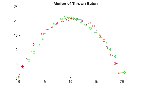
Plot Results
The output from solve contains the solutions of the equations of motion at each requested time step. To examine the results, plot the motion of the baton over time.
Loop through each column of the solution, and at each time step, plot the position of the baton. Color each end of the baton differently so that you can see its rotation over time.
figure
title("Motion of Thrown Baton");
axis([0 22 0 25])
hold on
for j = 1:length(sol.Time)
   theta = sol.Solution(5,j);
   X = sol.Solution(1,j);
   Y = sol.Solution(3,j);
   xvals = [X X+P(3)*cos(theta)];
   yvals = [Y Y+P(3)*sin(theta)];
   plot(xvals,yvals,xvals(1),yvals(1),"ro",xvals(2),yvals(2),"go")
end
hold off
References
[1] Wells, Dare A. Schaum’s Outline of Theory and Problems of Lagrangian Dynamics: With a Treatment of Euler’s Equations of Motion, Hamilton’s Equations and Hamilton’s Principle. Schaum's Outline Series. New York: Schaum Pub. Co, 1967.