Main Content

particleFilter

Particle filter object for online state estimation

Description

A particle filter is a recursive, Bayesian state estimator that uses discrete particles to approximate the posterior distribution of an estimated state. It is useful for online state estimation when measurements and a system model, that relates model states to the measurements, are available. The particle filter algorithm computes the state estimates recursively and involves initialization, prediction, and correction steps.

particleFilter creates an object for online state estimation of a discrete-time nonlinear system using the discrete-time particle filter algorithm.

Consider a plant with states x, input u, output m, process noise w, and measurement y. Assume that you can represent the plant as a nonlinear system.

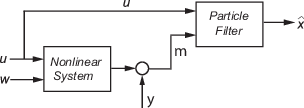
The algorithm computes the state estimates x^ of the nonlinear system using the state transition and measurement likelihood functions you specify.

The software supports arbitrary nonlinear state transition and measurement models, with arbitrary process and measurement noise distributions.

To perform online state estimation, create the nonlinear state transition function and measurement likelihood function. Then construct the particleFilter object using these nonlinear functions. After you create the object:

  1. Initialize the particles using the initialize command.

  2. Predict state estimates at the next step using the predict command.

  3. Correct the state estimates using the correct command.

The prediction step uses the latest state to predict the next state based on the state transition model you provide. The correction step uses the current sensor measurement to correct the state estimate. The algorithm optionally redistributes, or resamples, the particles in the state space to match the posterior distribution of the estimated state. Each particle represents a discrete state hypothesis of these state variables. The set of all particles is used to help determine the state estimate.

Creation

Object Description

example

pf = particleFilter(StateTransitionFcn,MeasurementLikelihoodFcn) creates a particle filter object for online state estimation of a discrete-time nonlinear system. StateTransitionFcn is a function that calculates the particles (state hypotheses) at the next time step, given the state vector at a time step. MeasurementLikelihoodFcn is a function that calculates the likelihood of each particle based on sensor measurements.

After creating the object, use the initialize command to initialize the particles with a known mean and covariance or uniformly distributed particles within defined bounds. Then, use the correct and predict commands to update particles (and hence the state estimate) using sensor measurements.

Input Arguments

expand all

State transition function, specified as a function handle, determines the transition of particles (state hypotheses) between time steps. Also a property of the particleFilter object. For more information, see Properties.

Measurement likelihood function, specified as a function handle, is used to calculate the likelihood of particles (state hypotheses) from sensor measurements. Also a property of the particleFilter object. For more information, see Properties.

Properties

expand all

Number of state variables, specified as a scalar. This property is read-only and is set using initialize. The number of states is implicit based on the specified matrices for the initial mean of particles, or the state bounds.

Number of particles used in the filter, specified as a scalar. Each particle represents a state hypothesis. You specify this property only by using initialize.

State transition function, specified as a function handle, determines the transition of particles (state hypotheses) between time steps. This function calculates the particles at the next time step, including the process noise, given particles at a time step.

In contrast, the state transition function for the extendedKalmanFilter and unscentedKalmanFilter generates a single state estimate at a given time step.

You write and save the state transition function for your nonlinear system, and specify it as a function handle when constructing the particleFilter object. For example, if vdpParticleFilterStateFcn.m is the state transition function, specify StateTransitionFcn as @vdpParticleFilterStateFcn. You can also specify StateTransitionFcn as a function handle to an anonymous function.

The function signature is as follows:

function predictedParticles = myStateTransitionFcn(previousParticles,varargin)

The StateTransitionFcn function accepts at least one input argument. The first argument is the set of particles previousParticles that represents the state hypotheses at the previous time step. The optional use of varargin in the function enables you to input any extra parameters that are relevant for predicting the next state, using predict, as follows:

predict(pf,arg1,arg2)

If StateOrientation is 'column', then previousParticles is a NumStateVariables-by-NumParticles array. If StateOrientation is 'row', then previousParticles is a NumParticles-by-NumStateVariables array.

StateTransitionFcn must return exactly one output, predictedParticles, which is the set of predicted particle locations for the current time step (array with same dimensions as previousParticles).

StateTransitionFcn must include the random process noise (from any distribution suitable for your application) in the predictedParticles.

To see an example of a state transition function with the StateOrientation property set to 'column', type edit vdpParticleFilterStateFcn at the command line.

Measurement likelihood function, specified as a function handle, is used to calculate the likelihood of particles (state hypotheses) using the sensor measurements. For each state hypothesis (particle), the function first calculates an N-element measurement hypothesis vector. Then the likelihood of each measurement hypothesis is calculated based on the sensor measurement and the measurement noise probability distribution.

In contrast, the measurement function for extendedKalmanFilter and unscentedKalmanFilter takes a single state hypothesis and returns a single measurement estimate.

You write and save the measurement likelihood function based on your measurement model, and use it to construct the object. For example, if vdpMeasurementLikelihoodFcn.m is the measurement likelihood function, specify MeasurementLikelihoodFcn as @vdpMeasurementLikelihoodFcn. You can also specify MeasurementLikelihoodFcn as a function handle to an anonymous function.

The function signature is as follows:

function likelihood = myMeasurementLikelihoodFcn(predictedParticles,measurement,varargin)

The MeasurementLikelihoodFcn function accepts at least two input arguments. The first argument is the set of particles predictedParticles that represents the predicted state hypothesis. If StateOrientation is 'column', then predictedParticles is a NumStateVariables-by-NumParticles array. If StateOrientation is 'row', then predictedParticles is a NumParticles-by-NumStateVariables array. The second argument, measurement, is the N-element sensor measurement at the current time step. You can provide additional input arguments using varargin.

The MeasurementLikelihoodFcn must return exactly one output, likelihood, a vector with NumParticles length, which is the likelihood of the given measurement for each particle (state hypothesis).

To see an example of a measurement likelihood function, type edit vdpMeasurementLikelihoodFcn at the command line.

Whether the state variables have a circular distribution, specified as a logical array.

This is a read-only property and is set using initialize.

Circular (or angular) distributions use a probability density function with a range of [-pi,pi]. IsStateVariableCircular is a row-vector with NumStateVariables elements. Each vector element indicates whether the associated state variable is circular.

Policy settings that determine when to trigger resampling, specified as a particleResamplingPolicy object.

The resampling of particles is a vital step in estimating states using a particle filter. It enables you to select particles based on the current state, instead of using the particle distribution given at initialization. By continuously resampling the particles around the current estimate, you can get more accurate tracking and improve long-term performance.

You can trigger resampling either at fixed intervals or dynamically, based on the number of effective particles. The minimum effective particle ratio is a measure of how well the current set of particles approximates the posterior distribution. The number of effective particles is calculated by:

Neff=1i=1N(wi)2

In this equation, N is the number of particles, and w is the normalized weight of each particle. The effective particle ratio is then Neff / NumParticles. Therefore, the effective particle ratio is a function of the weights of all the particles. After the weights of the particles reach a low enough value, they are not contributing to the state estimation. This low value triggers resampling, so the particles are closer to the current state estimation and have higher weights.

The following properties of the particleResamplingPolicy object can be modified to control when resampling is triggered:

PropertyValueTypeDescription

TriggerMethod

'ratio' (default)

'interval'

character vector

It is a method to determine when resampling occurs, based on the value chosen. The 'interval' value triggers resampling at regular time steps of the particle filter operation. The 'ratio' value triggers resampling based on the ratio of effective total particles.

SamplingInterval

1 (default)

scalar

Fixed interval between resampling, specified as a scalar. This interval determines during which correction steps the resampling is executed. For example, a value of 2 means the resampling is executed every second correction step. A value of inf means that resampling is never executed.

This property only applies with the TriggerMethod is set to 'interval'.

MinEffectiveParticleRatio

0.5 (default)

scalar

It is the minimum desired ratio of the effective number of particles to the total number of particles NumParticles. The effective number of particles is a measure of how well the current set of particles approximates the posterior distribution. A lower effective particle ratio implies that a lower number of particles are contributing to the estimation and resampling is required.

If the ratio of the effective number of particles to the total number of particles NumParticles falls below the MinEffectiveParticleRatio, a resampling step is triggered.

Method used for particle resampling, specified as one of the following:

  • 'multinomial' — Multinomial resampling, also called simplified random sampling, generates N random numbers independently from the uniform distribution in the open interval (0,1) and uses them to select particles proportional to their weight.

  • 'residual' — Residual resampling consists of two stages. The first stage is a deterministic replication of each particle that have weights larger than 1/N. The second stage consists of random sampling using the remainder of the weights (labelled as residuals).

  • 'stratified' — Stratified resampling divides the whole population of particles into subsets called strata. It pre-partitions the (0,1) interval into N disjoint sub-intervals of size 1/N. The random numbers are drawn independently in each of these sub-intervals and the sample indices chosen in the strata.

  • 'systematic' — Systematic resampling is similar to stratified resampling as it also makes use of strata. One distinction is that it only draws one random number from the open interval (0,1/N) and the remaining sample points are calculated deterministically at a fixed 1/N step size.

Method used for extracting a state estimate from particles, specified as one of the following:

  • 'mean' - The object outputs the weighted mean of the particles, depending on the properties Weights and Particles, as the state estimate.

  • 'maxweight' - The object outputs the particle with the highest weight as the state estimate.

Array of particle values, specified as an array based on the StateOrientation property:

  • If StateOrientation is 'row' then Particles is an NumParticles-by-NumStateVariables array.

  • If StateOrientation is 'column' then Particles is an NumStateVariables-by-NumParticles array.

Each row or column corresponds to a state hypothesis (a single particle).

Particle weights, defined as a vector based on the value of the StateOrientation property:

  • If StateOrientation is 'row' then Weights is a NumParticles-by-1 vector, where each weight is associated with the particle in the same row in the Particles property.

  • If StateOrientation is 'column' then Weights is a 1-by-NumParticles vector, where each weight is associated with the particle in the same column in the Particles property.

Current state estimate, defined as a vector based on the value of the StateOrientation property:

  • If StateOrientation is 'row' then State is a 1-by-NumStateVariables vector

  • If StateOrientation is 'column' then State is a NumStateVariables-by-1 vector

State is a read-only property, and is derived from Particles based on the StateEstimationMethod property. Refer to StateEstimationMethod for details on how the value of State is determined.

State along with StateCovariance can also be determined using getStateEstimate.

Current estimate of state estimation error covariance, defined as an NumStateVariables-by-NumStateVariables array. StateCovariance is a read-only property and is calculated based on the StateEstimationMethod. If you specify a state estimation method that does not support covariance, then the function returns StateCovariance as [ ].

StateCovariance and State can be determined together using getStateEstimate.

Object Functions

initializeInitialize the state of the particle filter
predictPredict state and state estimation error covariance at next time step using extended or unscented Kalman filter, or particle filter
correctCorrect state and state estimation error covariance using extended or unscented Kalman filter, or particle filter and measurements
getStateEstimateExtract best state estimate and covariance from particles
cloneCopy online state estimation object

Examples

collapse all

To create a particle filter object for estimating the states of your system, create appropriate state transition function and measurement likelihood function for the system.

In this example, the function vdpParticleFilterStateFcn describes a discrete-time approximation to van der Pol oscillator with nonlinearity parameter, mu, equal to 1. In addition, it models Gaussian process noise. vdpMeasurementLikelihood function calculates the likelihood of particles from the noisy measurements of the first state, assuming a Gaussian measurement noise distribution.

Create the particle filter object. Use function handles to provide the state transition and measurement likelihood functions to the object.

myPF = particleFilter(@vdpParticleFilterStateFcn,@vdpMeasurementLikelihoodFcn);

To initialize and estimate the states and state estimation error covariance from the constructed object, use the initialize, predict, and correct commands.

Load the van der Pol ODE data, and specify the sample time.

vdpODEdata.mat contains a simulation of the van der Pol ODE with nonlinearity parameter mu=1, using ode45, with initial conditions [2;0]. The true state was extracted with sample time dt = 0.05.

load ('vdpODEdata.mat','xTrue','dt')
tSpan = 0:dt:5;

Get the measurements. For this example, a sensor measures the first state with a Gaussian noise with standard deviation 0.04.

sqrtR = 0.04;
yMeas = xTrue(:,1) + sqrtR*randn(numel(tSpan),1);

Create a particle filter, and set the state transition and measurement likelihood functions.

myPF = particleFilter(@vdpParticleFilterStateFcn,@vdpMeasurementLikelihoodFcn);

Initialize the particle filter at state [2; 0] with unit covariance, and use 1000 particles.

initialize(myPF,1000,[2;0],eye(2));

Pick the mean state estimation and systematic resampling methods.

myPF.StateEstimationMethod = 'mean';
myPF.ResamplingMethod = 'systematic';

Estimate the states using the correct and predict commands, and store the estimated states.

xEst = zeros(size(xTrue));
for k=1:size(xTrue,1)
    xEst(k,:) = correct(myPF,yMeas(k));
    predict(myPF);
end

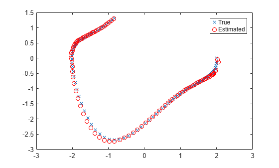
Plot the results, and compare the estimated and true states.

figure(1)
plot(xTrue(:,1),xTrue(:,2),'x',xEst(:,1),xEst(:,2),'ro')
legend('True','Estimated')

Figure contains an axes object. The axes object contains 2 objects of type line. One or more of the lines displays its values using only markers These objects represent True, Estimated.

References

[1] T. Li, M. Bolic, P.M. Djuric, "Resampling Methods for Particle Filtering: Classification, implementation, and strategies," IEEE Signal Processing Magazine, vol. 32, no. 3, pp. 70-86, May 2015.

Extended Capabilities

Version History

Introduced in R2017b