Main Content

extendedKalmanFilter

Create extended Kalman filter object for online state estimation

Description

extendedKalmanFilter creates an object for online state estimation of a discrete-time nonlinear system using the first-order discrete-time extended Kalman filter algorithm.

When you perform online state estimation, you first create the nonlinear state transition function f and measurement function h. You then construct the extendedKalmanFilter object using these nonlinear functions, and specify whether the noise terms are additive or nonadditive. You can also specify the Jacobians of the state transition and measurement functions by either generating them using automatic differentiation in the generateJacobianFcn function or by writing them yourself. If you do not specify them, the software numerically computes the Jacobians.

After you create the object, you use the predict command to predict state estimate at the next time step, and correct to correct state estimates using the algorithm and real-time data. For information about the algorithm, see Algorithms.

Creation

Description

example

obj = extendedKalmanFilter(stateTransitionFcn,measurementFcn,initialState) creates an extended Kalman filter object for online state estimation of a discrete-time nonlinear system.

  • stateTransitionFcn is a function that calculates the state of the system at time k, given the state vector at time k-1. This function is stored in the StateTransitionFcn property of the object.

  • measurementFcn is a function that calculates the output measurement of the system at time k, given the state at time k. This function is stored in the MeasurementFcn property of the object.

  • initialState specifies the initial value of the state estimates. This value is stored in the State property of the object.

After creating the object, use the correct and predict functions to update state estimates and state estimation error covariance values using a first-order discrete-time extended Kalman filter algorithm and real-time data.

  • predict updates obj.State and obj.StateCovariance with the predicted value at time step k using the state value at time step k–1.

  • correct updates obj.State and obj.StateCovariance with the estimated values at time step k using measured data at time step k.

example

obj = extendedKalmanFilter(___,Name,Value) additionally sets properties using name-value arguments. If you do not specify the state transition function, measurement function, and initial state values during creation, specify them using dot notation. For example, for a two-state system with initial state values [1;0], to specify these values after creation, use obj.State = [1;0].

Properties

expand all

extendedKalmanFilter object properties are of three types:

  • Tunable properties that you can specify multiple times, either during object construction using name-value arguments, or any time afterward during state estimation. After object creation, use dot notation to modify the tunable properties.

    obj = extendedKalmanFilter(StateTransitionFcn,MeasurementFcn,InitialState);
    obj.ProcessNoise = 0.01;

    The tunable properties are State, StateCovariance, ProcessNoise, and MeasurementNoise.

  • Nontunable properties that you can specify once, either during object construction or afterward using dot notion. Specify these properties before state estimation using correct and predict. The StateTransitionFcn, MeasurementFcn, StateTransitionJacobianFcn, and MeasurementJacobianFcn properties belong to this category.

  • Nontunable properties that you must specify during object construction. The HasAdditiveProcessNoise and HasAdditiveMeasurementNoise properties belong to this category.

Measurement noise characteristics, specified as one of the following values:

  • true — Measurement noise v is additive. The measurement function h that is specified in MeasurementFcn has the following form:

    y(k) = h(x(k),Um1,...,Umn)

    Where y(k) and x(k) are the estimated output and estimated state at time k, and Um1,...,Umn are any optional input arguments required by your measurement function.

  • false — Measurement noise is nonadditive. The measurement function specifies how the output measurement evolves as a function of the state and measurement noise:

    y(k) = h(x(k),v(k),Um1,...,Umn)

HasAdditiveMeasurementNoise is a nontunable property, and you can specify it only during object construction. You cannot change it using dot notation.

Process noise characteristics, specified as one of the following values:

  • true — Process noise w is additive. The state transition function f specified in StateTransitionFcn has the following form:

    x(k) = f(x(k-1),Us1,...,Usn)

    Where x(k) is the estimated state at time k, and Us1,...,Usn are any additional input arguments required by your state transition function.

  • false — Process noise is nonadditive. The state transition function specifies how the states evolve as a function of the state and process noise at the previous time step:

    x(k) = f(x(k-1),w(k-1),Us1,...,Usn)

HasAdditiveProcessNoise is a nontunable property, and you can specify it only during object construction. You cannot change it using dot notation.

Measurement function h, specified as a function handle. The function calculates the N-element output measurement vector of the nonlinear system at time step k, given the state vector at time step k. N is the number of measurements of the system. You write and save the measurement function and use it to construct the object. For example, if vdpMeasurementFcn.m is the measurement function, specify MeasurementFcn as @vdpMeasurementFcn. You can also specify MeasurementFcn as a function handle to an anonymous function.

The inputs to the function depend on whether you specify the measurement noise as additive or nonadditive in the HasAdditiveMeasurementNoise property of the object:

  • HasAdditiveMeasurementNoise is true — The measurement noise v is additive, and the measurement function specifies how the measurements evolve as a function of state values:

    y(k) = h(x(k),Um1,...,Umn)

    Where y(k) and x(k) are the estimated output and estimated state at time k, and Um1,...,Umn are any optional input arguments required by your measurement function. For example, if you are using multiple sensors for tracking an object, an additional input could be the sensor position. During estimation, you pass these additional arguments to the correct command which in turn passes them to the measurement function.

  • HasAdditiveMeasurementNoise is false — The measurement noise is nonadditive, and the measurement function also specifies how the output measurement evolves as a function of the measurement noise:

    y(k) = h(x(k),v(k),Um1,...,Umn)

When you have the HasMeasurementWrapping property enabled, then the output for the measurement function must also include the wrapping bounds, specified as an N-by-2 matrix, where the first column provides the minimum measurement bound and the second column provides the maximum measurement bound. N is the number of measurements of the system.

To see an example of a measurement function with additive process noise, enter edit vdpMeasurementFcn at the command line. To see an example of a measurement function with nonadditive process noise, enter edit vdpMeasurementNonAdditiveNoiseFcn.

MeasurementFcn is a nontunable property. You can specify it once before you use the correct command, either during object construction or using dot notation after object construction. You cannot change it after using the correct command.

Jacobian of measurement function h, specified as one of the following:

  • [] — The Jacobian is numerically computed at every call to the correct command. This can increase processing time and numerical inaccuracy of the state estimation.

  • function handle — You either write and save the Jacobian function or generate the Jacobian function using generateJacobianFcn, and specify the handle to the function. For example, if vdpMeasurementJacobianFcn.m is the Jacobian function, specify MeasurementJacobianFcn as @vdpMeasurementJacobianFcn.

    The function calculates the partial derivatives of the measurement function with respect to the states and measurement noise. The number of inputs to the Jacobian function must equal the number of inputs to the measurement function and must be specified in the same order in both functions. The number of outputs of the Jacobian function depends on the HasAdditiveMeasurementNoise property:

    • HasAdditiveMeasurementNoise is true — The function calculates the partial derivatives of the measurement function with respect to the states (h/x). The output is as an N-by-Ns Jacobian matrix, where N is the number of measurements of the system and Ns is the number of states.

    • HasAdditiveMeasurementNoise is false — The function also returns a second output that is the partial derivative of the measurement function with respect to the measurement noise terms (h/v). The second output is returned as an N-by-V Jacobian matrix, where V is the number of measurement noise terms.

To see an example of a Jacobian function for additive measurement noise, enter edit vdpMeasurementJacobianFcn at the command line.

MeasurementJacobianFcn is a nontunable property. You can specify it once before you use the correct command, either during object construction or using dot notation after object construction. You cannot change it after using the correct command.

Measurement noise covariance, specified as a scalar or matrix depending on the value of the HasAdditiveMeasurementNoise property:

  • HasAdditiveMeasurementNoise is true — Specify the covariance as a scalar or an N-by-N matrix, where N is the number of measurements of the system. Specify a scalar if there is no cross-correlation between measurement noise terms and all the terms have the same variance. The software uses the scalar value to create an N-by-N diagonal matrix.

  • HasAdditiveMeasurementNoise is false — Specify the covariance as a V-by-V matrix, where V is the number of measurement noise terms. MeasurementNoise must be specified before using correct. After you specify MeasurementNoise as a matrix for the first time, to then change MeasurementNoise you can also specify it as a scalar. Specify as a scalar if there is no cross-correlation between the measurement noise terms and all the terms have the same variance. The software extends the scalar to a V-by-V diagonal matrix with the scalar on the diagonals.

MeasurementNoise is a tunable property. You can change it using dot notation.

Process noise covariance, specified as a scalar or matrix depending on the value of the HasAdditiveProcessNoise property:

  • HasAdditiveProcessNoise is true — Specify the covariance as a scalar or an Ns-by-Ns matrix, where Ns is the number of states of the system. Specify a scalar if there is no cross-correlation between process noise terms, and all the terms have the same variance. The software uses the scalar value to create an Ns-by-Ns diagonal matrix.

  • HasAdditiveProcessNoise is false — Specify the covariance as a W-by-W matrix, where W is the number of process noise terms. ProcessNoise must be specified before using predict. After you specify ProcessNoise as a matrix for the first time, to then change ProcessNoise you can also specify it as a scalar. Specify as a scalar if there is no cross-correlation between the process noise terms and all the terms have the same variance. The software extends the scalar to a W-by-W diagonal matrix.

ProcessNoise is a tunable property. You can change it using dot notation.

State of the nonlinear system, specified as a vector of size Ns, where Ns is the number of states of the system.

When you use the predict command, State is updated with the predicted value at time step k using the state value at time step k–1. When you use the correct command, State is updated with the estimated value at time step k using measured data at time step k.

The initial value of State is the value you specify in the InitialState input argument during object creation. If you specify InitialState as a column vector, then State is also a column vector, and the predict and correct commands return state estimates as a column vector. Otherwise, a row vector is returned. If you want a filter with single-precision floating-point variables, you must specify State as a single-precision variable during object construction using the InitialState input argument.

State is a tunable property. You can change it using dot notation.

State estimation error covariance, specified as a scalar or an Ns-by-Ns matrix, where Ns is the number of states of the system. If you specify a scalar, the software uses the scalar value to create an Ns-by-Ns diagonal matrix.

Specify a high value for the covariance when you do not have confidence in the initial state values that you specify in the InitialState input argument.

When you use the predict command, StateCovariance is updated with the predicted value at time step k using the state value at time step k–1. When you use the correct command, StateCovariance is updated with the estimated value at time step k using measured data at time step k.

StateCovariance is a tunable property. You can change it using dot notation after you use the correct or predict commands.

State transition function f, specified as a function handle. The function calculates the Ns-element state vector of the system at time step k, given the state vector at time step k-1. Ns is the number of states of the nonlinear system.

You write and save the state transition function for your nonlinear system and use it to construct the object. For example, if vdpStateFcn.m is the state transition function, specify StateTransitionFcn as @vdpStateFcn. You can also specify StateTransitionFcn as a function handle to an anonymous function.

The inputs to the function you write depend on whether you specify the process noise as additive or nonadditive in the HasAdditiveProcessNoise property of the object:

  • HasAdditiveProcessNoise is true — The process noise w is additive, and the state transition function specifies how the states evolve as a function of state values at previous time step:

    x(k) = f(x(k-1),Us1,...,Usn)

    Where x(k) is the estimated state at time k, and Us1,...,Usn are any additional input arguments required by your state transition function, such as system inputs or the sample time. During estimation, you pass these additional arguments to the predict command, which in turn passes them to the state transition function.

  • HasAdditiveProcessNoise is false — The process noise is nonadditive, and the state transition function also specifies how the states evolve as a function of the process noise:

    x(k) = f(x(k-1),w(k-1),Us1,...,Usn)

To see an example of a state transition function with additive process noise, enter edit vdpStateFcn at the command line.

StateTransitionFcn is a nontunable property. You can specify it once before you use the predict command, either during object construction or using dot notation after object construction. You cannot change it after using the predict command.

Jacobian of the state transition function f, specified as one of the following:

  • [] — The Jacobian is numerically computed at every call to the predict command. This can increase processing time and numerical inaccuracy of the state estimation.

  • function handle — You either write and save the Jacobian function or generate the Jacobian function using generateJacobianFcn, and specify the handle to the function. For example, if vdpStateJacobianFcn.m is the Jacobian function, specify StateTransitionJacobianFcn as @vdpStateJacobianFcn.

    The function calculates the partial derivatives of the state transition function with respect to the states and process noise. The number of inputs to the function must equal the number of inputs of the state transition function and must be specified in the same order in both functions. The number of outputs of the function depends on the HasAdditiveProcessNoise property:

    • HasAdditiveProcessNoise is true — The function calculates the partial derivative of the state transition function with respect to the states (f/x). The output is an Ns-by-Ns Jacobian matrix, where Ns is the number of states.

    • HasAdditiveProcessNoise is false — The function must also return a second output that is the partial derivative of the state transition function with respect to the process noise terms (f/w). The second output is returned as an Ns-by-W Jacobian matrix, where W is the number of process noise terms.

The extended Kalman filter algorithm uses the Jacobian to compute the state estimation error covariance.

To see an example of a Jacobian function for additive process noise, at the MATLAB® command prompt, enter the following:

edit vdpStateJacobianFcn

StateTransitionJacobianFcn is a nontunable property. You can specify it once before you use the predict command, either during object construction or using dot notation after object construction. You cannot change it after using the predict command.

Enable measurement wrapping, specified as either 0 or 1. You can enable measurement wrapping to estimate states when you have circular measurements that are independent of your model states. If you select this parameter, then the measurement function you specify must include the following two outputs:

  1. The measurement, specified as a N-element output measurement vector of the nonlinear system at time step k, given the state vector at time step k. N is the number of measurements of the system.

  2. The measurement wrapping bounds, specified as an N-by-2 matrix where, the first column provides the minimum measurement bound and the second column provides the maximum measurement bound.

Enabling the HasMeasurementWrapping property wraps the measurement residuals in a defined bound, which helps to prevent the filter from divergence due to incorrect measurement residual values. For an example, see State Estimation with Wrapped Measurements Using Extended Kalman Filter.

HasMeasurementWrapping is a nontunable property. You can specify it once during the object construction. You cannot change it after creating the state estimation object.

Object Functions

correctCorrect state and state estimation error covariance using extended or unscented Kalman filter, or particle filter and measurements
predictPredict state and state estimation error covariance at next time step using extended or unscented Kalman filter, or particle filter
residualReturn measurement residual and residual covariance when using extended or unscented Kalman filter
cloneCopy online state estimation object
generateJacobianFcnGenerate MATLAB Jacobian functions for extended Kalman filter using automatic differentiation

Examples

collapse all

To define an extended Kalman filter object for estimating the states of your system, you first write and save the state transition function and measurement function for the system.

In this example, use the previously written and saved state transition and measurement functions, vdpStateFcn.m and vdpMeasurementFcn.m. These functions describe a discrete-approximation to a van der Pol oscillator with nonlinearity parameter, mu, equal to 1. The oscillator has two states.

Specify an initial guess for the two states. You specify the guess as an M-element row or column vector, where M is the number of states.

initialStateGuess = [1;0];

Create the extended Kalman filter object. Use function handles to provide the state transition and measurement functions to the object.

obj = extendedKalmanFilter(@vdpStateFcn,@vdpMeasurementFcn,initialStateGuess);

The object has a default structure where the process and measurement noise are additive.

To estimate the states and state estimation error covariance from the constructed object, use the correct and predict commands and real-time data.

Create an extended Kalman filter object for a van der Pol oscillator with two states and one output. Use the previously written and saved state transition and measurement functions, vdpStateFcn.m and vdpMeasurementFcn.m. These functions are written for additive process and measurement noise terms. Specify the initial state values for the two states as [2;0].

Since the system has two states and the process noise is additive, the process noise is a 2-element vector and the process noise covariance is a 2-by-2 matrix. Assume there is no cross-correlation between process noise terms, and both the terms have the same variance 0.01. You can specify the process noise covariance as a scalar. The software uses the scalar value to create a 2-by-2 diagonal matrix with 0.01 on the diagonals.

Specify the process noise covariance during object construction.

obj = extendedKalmanFilter(@vdpStateFcn,@vdpMeasurementFcn,[2;0],...
    'ProcessNoise',0.01);

Alternatively, you can specify noise covariances after object construction using dot notation. For example, specify the measurement noise covariance as 0.2.

obj.MeasurementNoise = 0.2;

Since the system has only one output, the measurement noise is a 1-element vector and the MeasurementNoise property denotes the variance of the measurement noise.

Create an extended Kalman filter (EKF) object for a van der Pol oscillator with two states and one output. Use the previously written and saved state transition and measurement functions, vdpStateFcn.m and vdpMeasurementFcn.m. Specify the initial state values for the two states as [2;0].

obj = extendedKalmanFilter(@vdpStateFcn,@vdpMeasurementFcn,[2;0]);

The extended Kalman filter algorithm uses Jacobians of the state transition and measurement functions for state estimation. You can write and save the Jacobian functions and provide them as function handles to the EKF object. For this object, use the previously written and saved functions vdpStateJacobianFcn.m and vdpMeasurementJacobianFcn.m.

obj.StateTransitionJacobianFcn = @vdpStateJacobianFcn;
obj.MeasurementJacobianFcn = @vdpMeasurementJacobianFcn;

If the Jacobian functions are not available, you can generate them using automatic differentiation.

obj.StateTransitionJacobianFcn = generateJacobianFcn(obj,'state');
obj.MeasurementJacobianFcn = generateJacobianFcn(obj,'measurement');

If you do not specify the Jacobians of the functions, the software numerically computes them. This numerical computation can result in increased processing time and numerical inaccuracy of the state estimation.

Create an extended Kalman filter object for a van der Pol oscillator with two states and one output. Assume that the process noise terms in the state transition function are additive. That is, there is a linear relation between the state and process noise. Also assume that the measurement noise terms are nonadditive. That is, there is a nonlinear relation between the measurement and measurement noise.

obj = extendedKalmanFilter('HasAdditiveMeasurementNoise',false);

Specify the state transition function and measurement functions. Use the previously written and saved functions, vdpStateFcn.m and vdpMeasurementNonAdditiveNoiseFcn.m.

The state transition function is written assuming the process noise is additive. The measurement function is written assuming the measurement noise is nonadditive.

obj.StateTransitionFcn = @vdpStateFcn;
obj.MeasurementFcn = @vdpMeasurementNonAdditiveNoiseFcn;

Specify the initial state values for the two states as [2;0].

obj.State = [2;0];

You can now use the correct and predict commands to estimate the state and state estimation error covariance values from the constructed object.

Consider a nonlinear system with input u whose state x and measurement y evolve according to the following state transition and measurement equations:

x[k]=x[k-1]+u[k-1]+w[k-1]

y[k]=x[k]+2*u[k]+v[k]2

The process noise w of the system is additive while the measurement noise v is nonadditive.

Create the state transition function and measurement function for the system. Specify the functions with an additional input u.

f = @(x,u)(sqrt(x+u));
h = @(x,v,u)(x+2*u+v^2);

f and h are function handles to the anonymous functions that store the state transition and measurement functions, respectively. In the measurement function, because the measurement noise is nonadditive, v is also specified as an input. Note that v is specified as an input before the additional input u.

Create an extended Kalman filter object for estimating the state of the nonlinear system using the specified functions. Specify the initial value of the state as 1 and the measurement noise as nonadditive.

obj = extendedKalmanFilter(f,h,1,'HasAdditiveMeasurementNoise',false);

Specify the measurement noise covariance.

obj.MeasurementNoise = 0.01;

You can now estimate the state of the system using the predict and correct commands. You pass the values of u to predict and correct, which in turn pass them to the state transition and measurement functions, respectively.

Correct the state estimate with measurement y[k]=0.8 and input u[k]=0.2 at time step k.

correct(obj,0.8,0.2)

Predict the state at the next time step, given u[k]=0.2.

predict(obj,0.2)

Retrieve the error, or residual, between the prediction and the measurement.

[Residual, ResidualCovariance] = residual(obj,0.8,0.2);

Algorithms

The first-order, discrete-time extended Kalman filter algorithm performs online state estimation of a discrete-time nonlinear system.

Consider a plant with states x, input u, output y, process noise w, and measurement noise v. Assume that you can represent the plant as a nonlinear system.

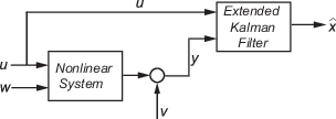
The algorithm computes the state estimates x^ of the nonlinear system using state transition and measurement functions specified by you. The software lets you specify the noise in these functions as additive or nonadditive:

  • Additive Noise Terms — The state transition and measurements equations have the following form:

    x[k]=f(x[k1],us[k1])+w[k1]y[k]=h(x[k],um[k])+v[k]

    Here f is a nonlinear state transition function that describes the evolution of states x from one time step to the next. The nonlinear measurement function h relates x to the measurements y at time step k. w and v are the zero-mean, uncorrelated process and measurement noises, respectively. These functions can also have additional input arguments that are denoted by us and um in the equations. For example, the additional arguments could be time step k or the inputs u to the nonlinear system. There can be multiple such arguments.

    Note that the noise terms in both equations are additive. That is, x(k) is linearly related to the process noise w(k-1), and y(k) is linearly related to the measurement noise v(k).

  • Nonadditive Noise Terms — The software also supports more complex state transition and measurement functions where the state x[k] and measurement y[k] are nonlinear functions of the process noise and measurement noise, respectively. When the noise terms are nonadditive, the state transition and measurements equation have the following form:

    x[k]=f(x[k1],w[k1],us[k1])y[k]=h(x[k],v[k],um[k])

When you perform online state estimation, you first create the nonlinear state transition function f and measurement function h. You then construct the extendedKalmanFilter object using these nonlinear functions, and specify whether the noise terms are additive or nonadditive. You can also specify the Jacobians of the state transition and measurement functions by either generating them using automatic differentiation in the generateJacobianFcn function or by writing them yourself. If you do not specify them, the software numerically computes the Jacobians.

After you create the object, you use the predict command to predict state estimate at the next time step, and correct to correct state estimates using the algorithm and real-time data. For additional details about the algorithm, see Extended and Unscented Kalman Filter Algorithms for Online State Estimation.

Extended Capabilities

Version History

Introduced in R2016b

expand all