Customize FIS Tuning Process
You can customize your FIS tuning process by either:
Specifying a custom cost function, which is supported for both Fuzzy Logic Designer and
tunefis. A custom cost function is useful for: (since R2023a)Training a FIS using a custom model in MATLAB® without using input/output training data. For an example, see Tune Fuzzy Robot Obstacle Avoidance System Using Custom Cost Function.
Training a FIS using a custom model implemented in Simulink®. This method is not supported for tuning FIS trees. For an example, see Design Controller for Artificial Pancreas Using Fuzzy Logic.
Combining the outputs of the component FISs of a FIS tree using mathematical operations, as shown in Tune FIS Using Custom Optimization Method.
Using a custom optimization method, which is supported only at the command line and does not use
tunefis. For an example, see Tune FIS Using Custom Cost Function.
For more information on tuning a FIS, see Tuning Fuzzy Inference Systems.
Specify Custom Cost Function in Fuzzy Logic Designer
Since R2023a
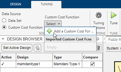
To specify a custom cost function when tuning a FIS using Fuzzy Logic Designer, on the Tuning tab, select Custom Cost Function.
Then, in the Custom Cost Function list, select Add a Custom Cost Fcn.
For this example, consider the following cost function,
myCostFcn, which simulates a Simulink model using the specified FIS.
The first input of the cost function is the FIS object, which is a required input.
The other inputs are the name of the Simulink model and the FIS variable name in the MATLAB workspace. Specifying additional inputs is optional.
The cost function updates the FIS variable in the workspace and simulates the model. It then extracts the reference and actual outputs from the model and computes the root mean squared error.
The output of the cost function is the scalar cost value, which in this case is the root mean squared error.
function cost = myCostFcn(fis,model,fisVarName)
% Evaluate model, generate output, and find the cost.

% Update workspace variable for the controller.
assignin('base',fisVarName,fis)

% Get simulation output.
out = sim(model);

% Get output and reference values from simulation output.
outVal = out.yout.signals(1).values;
refVal = out.yout.signals(2).values;
tout = out.yout.time;

% Calculate error from the nominal value.
err = outVal - refVal;

% Calculate cost as the root mean squared error.
cost = sqrt(mean(err.^2));

end
In the Add cost function dialog box, in the Function field, enter the name of your custom cost function. When you do so, the Required Inputs table shows the FIS input argument and the Additional Inputs table shows the other inputs.
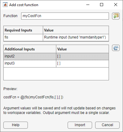
Specify values for the additional inputs by selecting previously defined variables from the MATLAB workspace. For this example:
input2corresponds to the Simulink model name. Select themodelNamevariable.input3corresponds to the FIS name in model workspace. Select thefisNamevariable.
The values of these variables are saved in the app with the cost function. Therefore, their values do not change when the variable in the MATLAB workspace changes. For this example, if the model name or FIS name change, you must add a new custom cost function in the app.
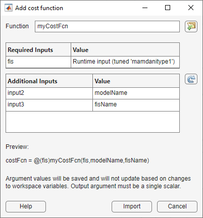
The dialog box shows a preview of the cost function signature. To add this cost function to the app, click Import.
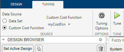
The app imports and selects the custom cost function.
Tune FIS Using Custom Cost Function
You can use a custom cost function to combine the outputs of the component FISs of a FIS tree using mathematical operations.
As an example, suppose that you want to create a FIS tree for approximating the function . You could implement a FIS tree that models all of the mathematical operations using component FIS objects, as shown in an example in tunefis.

However, to improve the FIS tree performance, you can create a FIS tree that combines the outputs of the component FIS objects using the known mathematical operations in the equation. Do create such a FIS tree, you must use a custom cost function during tuning.
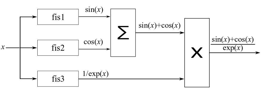
To tune a FIS tree for the second case, first create three FIS objects.
fis1 = sugfis(Name="fis1");
fis1 = addInput(fis1,[0 10], ...
    NumMFs=3, ...
    MFType="gaussmf");
fis1 = addOutput(fis1,[-1 1],NumMFs=3);

fis2 = sugfis(Name="fis2");
fis2 = addInput(fis2,[0 10], ...
    NumMFs=3, ...
    MFType="gaussmf");
fis2 = addOutput(fis2,[-1 1],NumMFs=3);

fis3 = sugfis(Name="fis3");
fis3 = addInput(fis3,[0 10], ...
    NumMFs=3, ...
    MFType="gaussmf");
fis3 = addOutput(fis3,[0 1],NumMFs=3);
Create a FIS tree where all three FIS objects have the same input and the outputs of the FIS tree are the outputs of the individual FIS objects.
con = ["fis1/input1" "fis2/input1";
       "fis2/input1" "fis3/input1"];

fisT = fistree([fis1 fis2 fis3],con);
Generate training data.
x = (0:0.1:10)';
y1 = sin(x)+cos(x);
y2 = y1./exp(x);
y = [y1 y2];
To implement the addition and multiplication operations, use a custom cost function. For this example, use the custom function customcostfcn, which is included at the end of the example. Learn a rule base using this cost function.
options = tunefisOptions(...
    Method="particleswarm", ...
    OptimizationType="learning");
options.MethodOptions.MaxIterations = 5;
rng("default")
fisTout1 = tunefis(fisT,[], ...
    @(fis)customcostfcn(fis,x,y),options);
                                 Best            Mean     Stall
Iteration     f-count            f(x)            f(x)    Iterations
    0             100           0.746            1.31        0
    1             200          0.5089           1.249        0
    2             300          0.5089           1.086        1
    3             400          0.5089           1.112        2
    4             500          0.5089           1.106        3
    5             600          0.4999           1.051        0
Optimization ended: number of iterations exceeded OPTIONS.MaxIterations.
Tune all the parameters of the FIS tree.
options.Method = "patternsearch";
options.MethodOptions.MaxIterations = 25;
[in,out,rule] = getTunableSettings(fisTout1);
fisTout2 = tunefis(fisTout1,[in;out;rule], ...
    @(fis)customcostfcn(fis,x,y),options);
Iter     Func-count       f(x)      MeshSize     Method
    0           1       0.499882             1
    1          17       0.499882             2     Successful Poll
    2          21       0.499882             1     Refine Mesh
    3          64       0.499882           0.5     Refine Mesh
    4         128       0.499882          0.25     Refine Mesh
    5         143       0.499309           0.5     Successful Poll
    6         206       0.499309          0.25     Refine Mesh
    7         216       0.497834           0.5     Successful Poll
    8         237        0.49493             1     Successful Poll
    9         279        0.49493           0.5     Refine Mesh
   10         341        0.49493          0.25     Refine Mesh
   11         405        0.49493         0.125     Refine Mesh
   12         463       0.490647          0.25     Successful Poll
   13         527       0.490647         0.125     Refine Mesh
   14         567       0.490257          0.25     Successful Poll
   15         631       0.490257         0.125     Refine Mesh
   16         673       0.486303          0.25     Successful Poll
   17         737       0.486303         0.125     Refine Mesh
   18         748       0.485744          0.25     Successful Poll
   19         812       0.485744         0.125     Refine Mesh
   20         884       0.485744        0.0625     Refine Mesh
   21         921       0.484482         0.125     Successful Poll
   22         932       0.484045          0.25     Successful Poll
   23         996       0.484045         0.125     Refine Mesh
   24        1067       0.484045        0.0625     Refine Mesh
   25        1080       0.483977         0.125     Successful Poll
   26        1151       0.483977        0.0625     Refine Mesh
patternsearch stopped because it exceeded options.MaxIterations.
Validate the trained system by evaluating the FIS tree using the input training data and comparing the result with the output training data.
Evaluate the FIS tree using the input training data.
yOut = evalfis(fisTout2,x);
Combine the outputs of the FIS tree using the known mathematical operations.
yResult = (yOut(:,1) + yOut(:,2)).*yOut(:,3);
Plot the results along with the output training data.
plot(x,y(:,2),"-",x,yResult,"-")
legend("Training Data","FIS Tree Output")

You can add more input/output MFs and specify additional FIS tree outputs to improve the tuning performance. Using additional MF parameters and more training data for additional FIS tree outputs can further fine-tune the outputs of fis1, fis2, and fis3.
Custom Cost Function
function cost = customcostfcn(fis,x,y)

tY = evalfis(fis,x);
sincosx = tY(:,1)+tY(:,2);
sincosexpx = sincosx.*tY(:,3);
actY = [sincosx;sincosexpx];
d = y(:)-actY;
cost = sqrt(mean(d.*d));

end
Tune FIS Using Custom Optimization Method
You can also implement your own FIS parameter optimization method using getTunableSettings, getTunableValues, and setTunableValues. This example uses these functions to tune a rule base of a fuzzy system.
Create a FIS to approximate , where varies from 0 to .
fisin = mamfis;
Add an input with a range of [0, ] and having five Gaussian MFs. Also, add an output with a range of [–1, 1] and having five Gaussian MFs.
fisin = addInput(fisin,[0 2*pi], ...
    NumMFs=5, ...
    MFType="gaussmf");
fisin = addOutput(fisin,[-1 1], ...
    NumMFs=5, ...
    MFType="gaussmf");
Add five rules.
rules = [1 1 1 1;
         2 2 1 1;
         3 3 1 1;
         4 4 1 1;
         5 5 1 1];
fisin = addRule(fisin,rules);
fisin.Rules
ans =
1×5 fisrule array with properties:
Description
Antecedent
Consequent
Weight
Connection
Details:
Description
________________________________
1 "input1==mf1 => output1=mf1 (1)"
2 "input1==mf2 => output1=mf2 (1)"
3 "input1==mf3 => output1=mf3 (1)"
4 "input1==mf4 => output1=mf4 (1)"
5 "input1==mf5 => output1=mf5 (1)"
For a faster FIS update, set DisableStructuralChecks to true.
fisin.DisableStructuralChecks = true;
Obtain the rule parameter settings.
[~,~,rule] = getTunableSettings(fisin);
Make the rule antecedents nontunable. In the rule consequents, do not allow NOT logic (negative MF indices) or empty variables (zero MF indices).
for i = 1:numel(rule)
    rule(i).Antecedent.Free = false;
    rule(i).Consequent.AllowNot = false;
    rule(i).Consequent.AllowEmpty = false;
end
Generate data for tuning.
x = (0:0.1:2*pi)';
y = sin(x);
To tune the rule parameters, use the custom function customtunefis included at the end of this example. Set the number of iterations to 2, and do not allow invalid parameter values when updating the FIS using setTunableValues.
numite = 2;
ignoreinvp = false;
fisout = customtunefis(fisin,rule,x,y,numite,ignoreinvp);
Initial cost = 1.170519
Iteration 1: Cost = 0.241121
Iteration 2: Cost = 0.241121
Display the tuned rules.
fisout.Rules
ans =
  1×5 fisrule array with properties:

    Description
    Antecedent
    Consequent
    Weight
    Connection

  Details:
                   Description
         ________________________________

    1    "input1==mf1 => output1=mf4 (1)"
    2    "input1==mf2 => output1=mf5 (1)"
    3    "input1==mf3 => output1=mf3 (1)"
    4    "input1==mf4 => output1=mf1 (1)"
    5    "input1==mf5 => output1=mf2 (1)"
Allow NOT logic in the rules and optimize the FIS again.
for i = 1:numel(rule)
    rule(i).Consequent.AllowNot = true;
end
fisout = customtunefis(fisin,rule,x,y,numite,ignoreinvp);
Initial cost = 1.170519
Iteration 1: Cost = 0.357052
Iteration 2: Cost = 0.241121
fisout.Rules
ans =
  1×5 fisrule array with properties:

    Description
    Antecedent
    Consequent
    Weight
    Connection

  Details:
                   Description
         ________________________________

    1    "input1==mf1 => output1=mf4 (1)"
    2    "input1==mf2 => output1=mf5 (1)"
    3    "input1==mf3 => output1=mf3 (1)"
    4    "input1==mf4 => output1=mf1 (1)"
    5    "input1==mf5 => output1=mf2 (1)"
Using NOT logic creates more combinations of rule parameters, resulting in more iterations to tune a FIS.
Next, reset AllowNot to false and set AllowEmpty to true. In other words, allow the absence of variables (zero output MF indices) in the consequents. Tune the FIS with the updated rule parameter settings.
for i = 1:numel(rule)
    rule(i).Consequent.AllowNot = false;
    rule(i).Consequent.AllowEmpty = true;
end

try
    fisout = customtunefis(fisin,rule,x,y,numite,ignoreinvp);
catch me
    disp("Error: " + me.message)
end
Initial cost = 1.170519
Error: Rule consequent must have at least one nonzero membership function index.
The tuning process fails since the FIS contains only one output, which must be nonzero (nonempty) in the rule consequent. To ignore invalid parameter values, specify IgnoreInvalidParameters with setTunableValues.
Set ignoreinvp to true, which specifies the IgnoreInvalidParameters value in the call to setTunableValues used in customtunefis.
ignoreinvp = true;
fisout = customtunefis(fisin,rule,x,y,numite,ignoreinvp);
Initial cost = 1.170519
Iteration 1: Cost = 0.241121
Iteration 2: Cost = 0.241121
fisout.Rules
ans =
  1×5 fisrule array with properties:

    Description
    Antecedent
    Consequent
    Weight
    Connection

  Details:
                   Description
         ________________________________

    1    "input1==mf1 => output1=mf4 (1)"
    2    "input1==mf2 => output1=mf5 (1)"
    3    "input1==mf3 => output1=mf3 (1)"
    4    "input1==mf4 => output1=mf1 (1)"
    5    "input1==mf5 => output1=mf2 (1)"
In this case, the tuning process bypasses the invalid values and uses only valid parameter values for optimization.
By default, tunefis ignores invalid values when updating fuzzy system parameters. You can change this behavior by setting tunefisOptions.IgnoreInvalidParameters to false.
Custom Functions
function fis = customtunefis(fis,rule,x,y,n,ignore)

% Show the initial cost.
cost = findcost(fis,x,y);
fprintf("Initial cost = %f\n",cost);

% Optimize the rule parameters.
numMFs = numel(fis.Outputs.MembershipFunctions);
for ite = 1:n
    for i = 1:numel(rule)
        % Get the consequent value.
        pval = getTunableValues(fis,rule(i));
        % Loop through the output MF indices to minimize the cost.
        % Use the output indices according to AllowNot and AllowEmpty.
        allowNot = rule(i).Consequent.AllowNot;
        allowEmpty = rule(i).Consequent.AllowEmpty;
        if allowNot && allowEmpty
            mfID = -numMFs:numMFs;
        elseif allowNot && ~allowEmpty
            mfID = [-numMFs:-1 1:numMFs];
        elseif ~allowNot && allowEmpty
            mfID = 0:numMFs;
        else
            mfID = 1:numMFs;
        end
        cost = 1000;
        minCostFIS = fis;
        for j = 1:length(mfID)
            % Update the consequent value.
            pval(1) = mfID(j);
            % Set the consequent value in the FIS.
            fis = setTunableValues(fis,rule(i), ...
                pval,IgnoreInvalidParameters=ignore);
            % Evaluate cost.
            rmse = findcost(fis,x,y);
            % Update the FIS with the minimum cost.
            if rmse<cost
                cost = rmse;
                minCostFIS = fis;
            end
        end
        fis = minCostFIS;
    end
    fprintf("Iteration %d: Cost = %f\n",ite,cost);
end

end
function cost = findcost(fis,x,y)

actY = evalfis(fis,x);
d = y - actY;
cost = sqrt(mean(d.*d));

end