Autonomous Underwater Vehicle Pose Estimation Using Inertial Sensors and Doppler Velocity Log
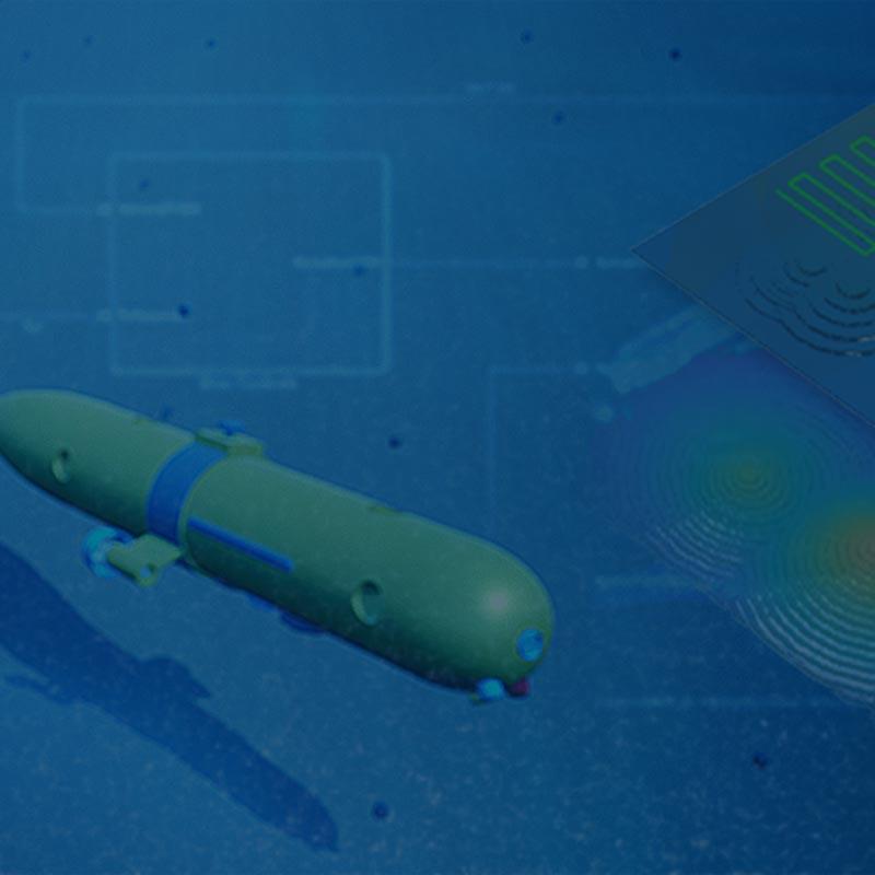
This example shows how to fuse data from a GPS, Doppler Velocity Log (DVL), and inertial measurement unit (IMU) sensors to estimate the pose of an autonomous underwater vehicle (AUV) shown in this image.
Background
A DVL sensor is capable of measuring the velocity of an underwater vehicle when it is close to the sea floor. Conversely, the GPS sensor can measure the position and velocity of the vehicle while it is near the surface using visible satellites. The IMU sensor aids these two sensors in pose estimation.
While the AUV is diving, there is a period when neither GPS nor DVL can be used because the GPS satellites cannot be reached and the sea floor is not within a scannable distance, requiring the IMU alone to estimate the pose. Even when using a high-quality IMU, such as a fiber-optic or ring-laser gyroscope, the pose estimate still accrues error when using the IMU by itself.
The lack of a second orientation sensor, such as a magnetometer, results in an inferior yaw estimate for the AUV relative to the pitch and roll estimates. This is because the IMU uses both its gyroscope and accelerometer for pitch and roll estimates, but uses only the gyroscope for yaw estimates.
This example shows you how to combine the IMU, GPS, and DVL sensors in a pose estimation filter to mitigate IMU errors. Furthermore, it shows how to reduce the error by smoothing the entire filter estimate.
Setup
Set the seed of the random number generator (RNG) to ensure repeatable results. Then create an instance of the example helper object ExampleHelperAUVTrajectoryPlotter, which enables you to visualize the results.
rng(1)
plotter = ExampleHelperAUVTrajectoryPlotter;
Create Dive and Surface Trajectory
To understand the relationship between the sensors of the AUV and the drift, you need a simple trajectory for the AUV that acts as the ground truth for the pose of the AUV. Following the trajectory, the AUV should travel at the surface, dive near the sea floor, travel along the sea floor, and eventually resurface.
Design Trajectory
Because the sensor rates determine the trajectory, you must set the rates at which the IMU, GPS, and DVL sensors update for the sensor simulations.
imuRate = 200; % 200 Hz update rate for IMU sensor simulation.
gpsRate = 1;   % 1 Hz update rate for GPS sensor simulation.
dvlRate = 5;   % 5 Hz update rate for DVL sensor simulation.
Specify the sensor update rates to the exampleHelperDiveAndSurfaceTrajectory helper function to create the trajectory of the AUV. This trajectory is the ground truth to compare with the simulated sensor data. The function also returns the depths at which the GPS and DVL sensors have reliable measurements.
[imuTraj,gpsTraj,dvlTraj,gpsDepth,dvlDepth] = exampleHelperDiveAndSurfaceTrajectory(imuRate,gpsRate,dvlRate);
Note that the maximum dive depth for the AUV is 10 meters for this example. This small depth illustrates the effect of sensors dropping in and out of usage while keeping the trajectory small enough to enable faster filter tuning.
Store the ground truth trajectory in a timetable object to use for comparison and filter tuning.
groundTruth = timetable(imuTraj.Position, ...
                        imuTraj.Orientation, ...
                        VariableNames=["Position","Orientation"], ...
                        SampleRate=imuRate);
Visualize Trajectory
Use the visualizeTrajectory object function of the helper object to plot the ground-truth trajectory with the regions of operation for each sensor.
plotter.visualizeTrajectory(groundTruth,gpsDepth,dvlDepth);

Generate Sensor Data and Estimate Pose
Use the exampleHelperGenerateAUVSensorData helper function to generate sensor data for the IMU, GPS, and DVL sensors mounted on the AUV.
sensorData = exampleHelperGenerateAUVSensorData(imuTraj,imuRate,gpsTraj,gpsRate,dvlTraj,dvlRate,gpsDepth,dvlDepth);
To estimate the AUV pose, you must fuse the sensor data using a filter. In this case, use an extended Kalman Filter with some simulated measurement noise.
Load a tuned insEKF object filt and the sensor measurement noise tmn. For more information about how to tune the filter, see the Tune Pose Filter section.
load("auvPoseEstimationTunedFilter.mat","filt","tmn");
Use the estimateStates object function to obtain a filter estimate of the poses and a smoother estimate of the poses.
[poseEst,smoothEst] = estimateStates(filt,sensorData,tmn);
Show Results
Analyze the output of the filter and smoother using these:
Position RMS error of the filter estimate, with sensor operating regions.
Ground truth position, compared to the filter and smoother estimates.
Subplots of the ground truth and the smoother estimate.
Create a plot to show the position RMS error when various sensors are available.
plotter.plotPositionRMS(groundTruth,poseEst,gpsDepth,dvlDepth);
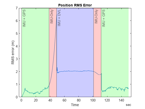
Note that the error increases when only the IMU is available for position estimation.
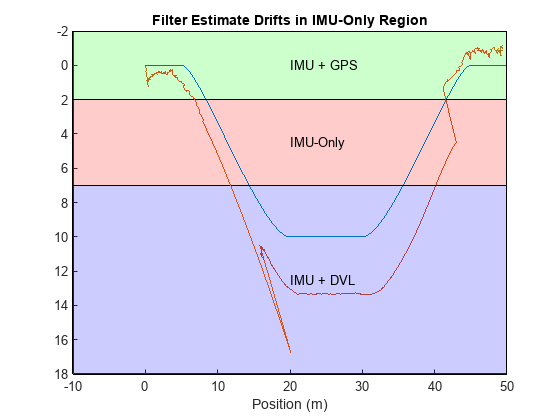
Plot the filter estimate and the ground truth together to compare the results. As seen in the previous plot, the estimate drifts when only the IMU is available. The filter corrects the drift when DVL measurements are available.
plotter.plotFilterEstimate(groundTruth,poseEst,gpsDepth,dvlDepth);
Compare the smoother estimate to the ground truth. The smoother removes the drift in the position states when only IMU is available.
plotter.plotSmootherEstimate(groundTruth,smoothEst,gpsDepth,dvlDepth);

Show the smoother position estimate over the entire trajectory, and compare it to the ground truth trajectory of the AUV.
plotter.animateEstimate(groundTruth,smoothEst,gpsDepth,dvlDepth);

Additional Information
The example showed how the differing regions of operation of each sensor on an AUV affect the accuracy of the pose estimation. These sections show the DVL sensor simulation model used in this example and how the insEKF object has been tuned.
DVL Simulation Model
This example models DVL beam velocities using this equation:
The simulation shown in the example performs a least-squares calculation to obtain the DVL-based velocity measurement of the vehicle. The DVL outputs NaN values when the vehicle is above the dvlDepth.
Tune Pose Filter
The example tunes the insEKF object using the exampleHelperTuneAUVPoseFilter helper function. To retune the filter, set the tuneFilter parameter to true.
The ExampleHelperINSDVL class is a simple sensor plugin that enables the insEKF to fuse DVL data.
classdef ExampleHelperINSDVL < positioning.INSSensorModel
%ExampleHelperINSDVL Template for sensor model using insEKF
%
%   This function is for use with AUVPoseEstimationIMUGPSDVLExample only.
%   It to be removed in the future.
%
%   See also insEKF, positioning.INSSensorModel.

%   Copyright 2022 The MathWorks, Inc.

    methods

        function z = measurement(~,filt)
            z = stateparts(filt,'Velocity');
        end

        function dzds = measurementJacobian(~,filt)

            N = numel(filt.State); % Number of states

            dzds = zeros(3,N,"like",filt.State);
            idx = stateinfo(filt,'Velocity');

            dzds(1,idx) = [1 0 0];
            dzds(2,idx) = [0 1 0];
            dzds(3,idx) = [0 0 1];
        end

    end
end
tuneFilter =false; if tuneFilter [filt,tmn] = exampleHelperTuneAUVPoseFilter(sensorData,groundTruth); %#ok<UNRCH> save("auvPoseEstimationTunedFilter.mat","filt","tmn"); end
You can also select a web site from the following list
Americas
- América Latina (Español)
- Canada (English)
- United States (English)
Europe
- Belgium (English)
- Denmark (English)
- Deutschland (Deutsch)
- España (Español)
- Finland (English)
- France (Français)
- Ireland (English)
- Italia (Italiano)
- Luxembourg (English)
- Netherlands (English)
- Norway (English)
- Österreich (Deutsch)
- Portugal (English)
- Sweden (English)
- Switzerland
- United Kingdom (English)
Asia Pacific
- Australia (English)
- India (English)
- New Zealand (English)
- 中国
- 日本Japanese (日本語)
- 한국Korean (한국어)