Square Jacobi SVD HDL Optimized

Libraries:
Fixed-Point Designer HDL Support /
Matrices and Linear Algebra /
Matrix Factorizations
Description
Use the Square Jacobi SVD HDL Optimized block to perform singular value
decomposition (SVD) on square matrices using the two-sided Jacobi algorithm. Given a square
matrix A, the Square Jacobi SVD HDL Optimized block uses the
two-sided Jacobi method to produce a vector s of nonnegative elements and
unitary matrices U and V such that A =
U*diag(s)*V'.
Note
For non-square matrices, use the Non-Square Jacobi SVD HDL Optimized block.
Examples
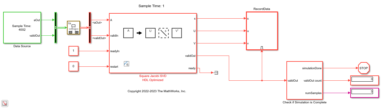
This example shows how to use the Square Jacobi SVD HDL Optimized block to compute the singular value decomposition (SVD) of square matrices.
Two-Sided Jacobi SVD
The Square Jacobi HDL Optimized block uses the two-sided Jacobi algorithm to perform singular value decomposition. Given an input square matrix A, the block first computes the two-by-two SVD for off-diagonal elements, then applies the rotation to the A, U, and V matrices. Because the Jacobi algorithm can perform such computations in parallel, it is suitable for FPGA and ASIC applications. For more information, see Square Jacobi SVD HDL Optimized.
Define Simulation Parameters
Specify the dimension of the sample matrices, the number of input sample matrices, and the number of iterations of the Jacobi algorithm.
n = 8;
numSamples = 3;
nIterations = 10;
Generate Input A Matrices
Use the specified simulation parameters to generate the input matrix A.
rng('default');
A = randn(n,n,numSamples);
The Square Jacobi SVD HDL Optimized block supports both real and complex inputs. Set the complexity of the input in the block mask accordingly.
% A = complex(randn(n,n,numSamples),randn(n,n,numSamples));
Select Fixed-Point Data Types
Define the desired word length.
wordLength = 32;
Use the upper bound on the singular values to define fixed-point types that will never overflow. First, use the fixed.singularValueUpperBound function to determine the upper bound on the singular values.
svdUpperBound = fixed.singularValueUpperBound(n,n,max(abs(A(:))));
Define the integer length based on the value of the upper bound, with one additional bit for the sign, another additional bit for intermediate CORDIC growth, and one more bit for intermediate growth to compute the Jacobi rotations.
additionalBitGrowth = 3;
integerLength = ceil(log2(svdUpperBound)) + additionalBitGrowth;
Compute the fraction length based on the integer length and the desired word length.
fractionLength = wordLength - integerLength;
Define the signed fixed-point data type to be 'Fixed' or 'ScaledDouble'. You can also define the type to be 'double' or 'single'.
dataType = 'Fixed';
T.A = fi([],1,wordLength,fractionLength,'DataType',dataType);
disp(T.A)
[]

          DataTypeMode: Fixed-point: binary point scaling
            Signedness: Signed
            WordLength: 32
        FractionLength: 24
Cast the matrix A to the signed fixed-point type.
A = cast(A,'like',T.A);
Configure Model Workspace and Run Simulation
model = 'SquareJacobiSVDModel';
open_system(model);
fixed.example.setModelWorkspace(model,'A',A,'n',n,...
    'nIterations',nIterations,'numSamples',numSamples);
out = sim(model);

Verify Output Solutions
Verify the output solutions. In these steps, "identical" means within roundoff error.
Verify that
U*diag(s)*V'is identical toA.relativeErrorUSVrepresents the relative error betweenU*diag(s)*V'andA.Verify that the singular values
sare identical to the floating-point SVD solution.relativeErrorSrepresents the relative error betweensand the singular values calculated by the MATLAB®svdfunction.Verify that
UandVare unitary matrices.relativeErrorUUrepresents the relative error betweenU'*Uand the identity matrix.relativeErrorVVrepresents the relative error betweenV'*Vand the identity matrix.
for i = 1:numSamples
    disp(['Sample #',num2str(i),':']);
    a = A(:,:,i);
    U = out.U(:,:,i);
    V = out.V(:,:,i);
    s = out.s(:,:,i);

    % Verify U*diag(s)*V'
    if norm(double(a)) > 1
        relativeErrorUSV = norm(double(U*diag(s)*V')-double(a))/norm(double(a));
    else
        relativeErrorUSV = norm(double(U*diag(s)*V')-double(a));
    end
    relativeErrorUSV %#ok

    % Verify s
    s_expected = svd(double(a));
    normS = norm(s_expected);
    relativeErrorS = norm(double(s) - s_expected);
    if normS > 1
        relativeErrorS = relativeErrorS/normS;
    end
    relativeErrorS %#ok

    % Verify U'*U
    U = double(U);
    UU = U'*U;
    relativeErrorUU = norm(UU - eye(size(UU))) %#ok

    % Verify V'*V
    V = double(V);
    VV = V'*V;
    relativeErrorVV = norm(VV - eye(size(VV))) %#ok

    disp('---------------');
end
Sample #1:

relativeErrorUSV =

   3.8655e-06


relativeErrorS =

   1.0144e-06


relativeErrorUU =

   2.6203e-07


relativeErrorVV =

   3.5127e-07

---------------
Sample #2:

relativeErrorUSV =

   4.9984e-06


relativeErrorS =

   1.3456e-06


relativeErrorUU =

   3.0184e-07


relativeErrorVV =

   3.7298e-07

---------------
Sample #3:

relativeErrorUSV =

   4.7606e-06


relativeErrorS =

   1.4317e-06


relativeErrorUU =

   4.2050e-07


relativeErrorVV =

   2.6215e-07

---------------
Extended Examples
Implement HDL Optimized SVD in Feedforward Fashion Without Backpressure
Implement a hardware-efficient singular value decomposition (SVD) using the Square Jacobi SVD HDL Optimized block in a feedforward fashion without backpressure.

Implement HDL Optimized SVD with Backpressure Signal and HDL FIFO Block
Implement hardware-efficient singular value decomposition (SVD) using the Square Jacobi SVD HDL Optimized block with backpressure control and an HDL FIFO block.
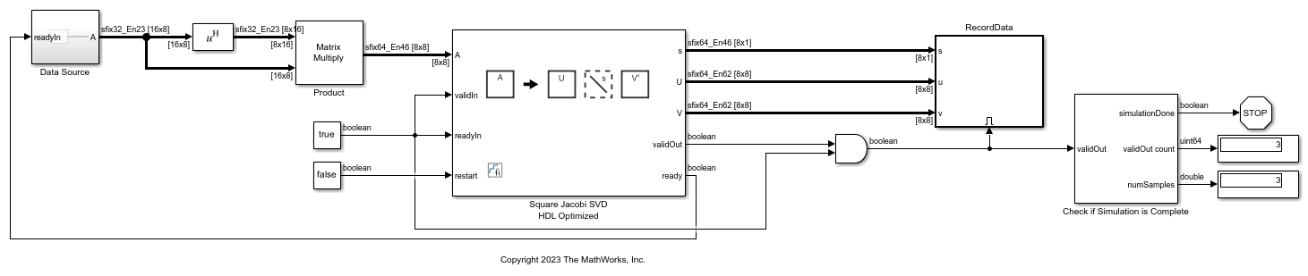
Compute SVD of Non-Square Matrices Using Square Jacobi SVD HDL Optimized Block by Forming Covariance Matrices
Use the Square Jacobi SVD HDL Optimized block to compute the singular value decomposition (SVD) of non-square matrices by forming covariance matrices.
Ports
Input
Output
Parameters
Tips
The Square Jacobi SVD HDL Optimized block computes the singular value decomposition in place. Set the fixed-point data type of the input
n-by-nmatrixAwith enough precision and enough headroom to avoid overflow.First, use the
fixed.singularValueUpperBoundfunction to determine the upper bound on the singular values. Then define the integer length based on the value of the upper bound, with one additional bit for the sign, another additional bit for intermediate CORDIC growth, and one more bit for intermediate growth to compute the Jacobi rotations. Compute the fraction length based on the integer length and the desired word length.svdUpperBound = fixed.singularValueUpperBound(n,n,max(abs(A(:)))) additionalBitGrowth = 3; integerLength = ceil(log2(svdUpperBound)) + additionalBitGrowth wordLength = 16 fractionLength = wordLength - integerLength
The behavior of the Square Jacobi SVD HDL Optimized block is equivalent to
[U,s,V] = fixed.jacobiSVD(A)whenAis a square matrix. If the input data type is fixed point with binary-point scaling, the function and the block provide bit-exact results. However, if the input data type is floating point, small numerical differences may exist between the function and the block.The Number of Jacobi iterations block parameter is equivalent to the
numberOfSweepsinput argument for thefixed.jacobiSVDfunction.The behavior of the Square Jacobi SVD HDL Optimized block is equivalent to
[U,s,V] =whenfixed.svd(A,'econ','vector')Ais a square matrix.
Algorithms
The latency of the Square Jacobi SVD HDL Optimized block depends on the
size (n), complexity, and word length (wl) of the
input matrix A, and the number of iterations
(nIterations) of the two-sided Jacobi algorithm, as summarized in the table.
If the data type of A is fixed point, then
wlis the word length.If the data type of A is double precision, then
wlis53.If the data type of A is single precision, then
wlis24.
| Signal Complexity | validIn to validOut |
|---|---|
Real |
(wl*2+31)*(n-1+rem(n,2))*nIterations+2+nextpow2(n)*(nextpow2(n)+1)/2+3 |
Complex |
(wl*6+48)*(n-1+rem(n,2))*nIterations+2+nextpow2(n)*(nextpow2(n)+1)/2+3 |
For example, assume that validIn asserts before
ready, meaning that the upstream data source is faster than the
Square Jacobi SVD HDL Optimized block. Additionally, assume that
readyIn is always asserted, meaning that the downstream consumer of the
data is faster than the Square Jacobi SVD HDL Optimized.

In the figure:
A1is the first A matrix,U1is the first U matrix,s1is the first s vector,V1is the first V matrix, and so on.validIntovalidOut— Goes from a successful matrix input to the block starting to output the solution.After a successful solution output, the block is ready again at the next clock cycle.
References
[1] Arm Developer. "AMBA AXI and ACE Protocol Specification Version E." https://developer.arm.com/documentation/ihi0022/e/.
[2] Jacobi, Carl G. J., "Über ein leichtes Verfahren die in der Theorie der Säcularstörungen vorkommenden Gleichungen numerisch aufzulösen." Journal fur die reine und angewandte Mathematik 30 (1846): 51–94.
[3] Forsythe, George E. and Peter Henrici. "The Cyclic Jacobi Method for Computing the Principal Values of a Complex Matrix." Transactions of the American Mathematical Society 94, no. 1 (January 1960): 1-23.
[4] Shiri, Aidin and Ghader Khosroshahi. "An FPGA Implementation of Singular Value Decomposition", ICEE 2019: 27th Iranian Conference on Electrical Engineering, Yazd, Iran, April 30–May 2, 2019, 416-22, IEEE.
[5] Golub, Gene H. and Charles F. Van Loan. Matrix Computations, 4th ed. Baltimore, MD: Johns Hopkins University Press, 2013.
[6] Athi, Mrudula V., Seyed R. Zekavat, and Alan A. Struthers. "Real-Time Signal Processing of Massive Sensor Arrays via a Parallel Fast Converging SVD Algorithm: Latency, Throughput, and Resource Analysis." IEEE Sensors Journal 16, no. 18 (January 2016): 2519-26. https://doi.org/10.1109/JSEN.2016.2517040.
[7] Brent, Richard P., Franklin T. Luk, and Charles Van Loan. "Computation of the Singular Value Decomposition Using Mesh-Connected Processors." Journal of VLSI and Computer Systems 1, 3 (1985): 242–70.
[8] Hemkumar, Nariankadu D. A Systolic VLSI Architecture for Complex SVD. Master’s thesis, Rice University, 1991.
[9] Duryea, R. A. Finite Precision Arithmetic in Singular Value Decomposition Architectures. Ph.D. thesis, Cornell University, 1987.
[10] Cavallaro, Joseph R. and Franklin T. Luk. 1987. "CORDIC Arithmetic for an SVD Processor." 1987 IEEE 8th Symposium on Computer Arithmetic (ARITH), Como, Italy, May 18-21, 1987, 113-20. IEEE. https://doi.org/10.1109/ARITH.1987.6158686.
Extended Capabilities
Version History
Introduced in R2023a