bininfo

Return predictor’s bin information

Syntax

bi = bininfo(sc,PredictorName)

bi = bininfo(___,Name,Value)

[bi,bm] = bininfo(sc,PredictorName,Name,Value)

[bi,bm,mv] = bininfo(sc,PredictorName,Name,Value)

Description

bi = bininfo(sc,PredictorName) returns information at bin level, such as frequencies of “Good,” “Bad,” and bin statistics for the predictor specified in PredictorName.

bi = bininfo(___,Name,Value) adds optional name-value arguments.

[bi,bm] = bininfo(sc,PredictorName,Name,Value) adds optional name-value arguments.bininfo also optionally returns the binning map (bm) or bin rules in the form of a vector of cut points for numeric predictors, or a table of category groupings for categorical predictors.

[bi,bm,mv] = bininfo(sc,PredictorName,Name,Value) returns information at bin level, such as frequencies of “Good,” “Bad," and bin statistics for the predictor specified in PredictorName using optional name-value pair arguments. bininfo optionally returns the binning map or bin rules in the form of a vector of cut points for numeric predictors, or a table of category groupings for categorical predictors. In addition, optional name-value pair arguments mv returns a numeric array containing the minimum and maximum values, as set (or defined) by the user. The mv output argument is set to an empty array for categorical predictors.

Examples

Display Bin Information Using Default Options

Create a creditscorecard object using the CreditCardData.mat file to load the data (using a dataset from Refaat 2011).

load CreditCardData 
sc = creditscorecard(data);

Display bin information for the categorical predictor ResStatus.

bi = bininfo(sc,'ResStatus')

bi=4×6 table
         Bin          Good    Bad     Odds        WOE       InfoValue
    ______________    ____    ___    ______    _________    _________

    {'Home Owner'}    365     177    2.0621     0.019329    0.0001682
    {'Tenant'    }    307     167    1.8383    -0.095564    0.0036638
    {'Other'     }    131      53    2.4717      0.20049    0.0059418
    {'Totals'    }    803     397    2.0227          NaN    0.0097738

Display Bin Information For a creditscorecard Object Containing Weights

Use the CreditCardData.mat file to load the data (dataWeights) that contains a column (RowWeights) for the weights (using a dataset from Refaat 2011).

load CreditCardData

Create a creditscorecard object using the optional name-value pair argument for 'WeightsVar'.

sc = creditscorecard(dataWeights,'WeightsVar','RowWeights')

sc = 
  creditscorecard with properties:

                GoodLabel: 0
              ResponseVar: 'status'
               WeightsVar: 'RowWeights'
                 VarNames: {'CustID'  'CustAge'  'TmAtAddress'  'ResStatus'  'EmpStatus'  'CustIncome'  'TmWBank'  'OtherCC'  'AMBalance'  'UtilRate'  'RowWeights'  'status'}
        NumericPredictors: {'CustID'  'CustAge'  'TmAtAddress'  'CustIncome'  'TmWBank'  'AMBalance'  'UtilRate'}
    CategoricalPredictors: {'ResStatus'  'EmpStatus'  'OtherCC'}
           BinMissingData: 0
                    IDVar: ''
            PredictorVars: {'CustID'  'CustAge'  'TmAtAddress'  'ResStatus'  'EmpStatus'  'CustIncome'  'TmWBank'  'OtherCC'  'AMBalance'  'UtilRate'}
                     Data: [1200×12 table]

Display bin information for the numerical predictor 'CustIncome'. When the optional name-value pair argument 'WeightsVar' is used to specify observation (sample) weights, the bi table contains weighted counts.

bi = bininfo(sc,'CustIncome');
bi(1:10,:)

ans=10×6 table
       Bin        Good        Bad       Odds        WOE       InfoValue 
    _________    _______    _______    _______    ________    __________

    {'18000'}    0.94515      1.496    0.63179     -1.1667     0.0059198
    {'19000'}    0.47588    0.80569    0.59065     -1.2341     0.0034716
    {'20000'}     2.1671     1.4636     1.4806    -0.31509    0.00061392
    {'21000'}     3.2522    0.88064      3.693     0.59889     0.0021303
    {'22000'}     1.5438     1.2714     1.2142    -0.51346     0.0012913
    {'23000'}      1.787     2.7529    0.64913     -1.1397      0.010509
    {'24000'}     3.4111     2.2538     1.5135    -0.29311    0.00082663
    {'25000'}     2.2333     6.1383    0.36383     -1.7186      0.042642
    {'26000'}     2.1246     4.4754    0.47474     -1.4525      0.024526
    {'27000'}     3.1058      3.528    0.88032    -0.83501     0.0082144

Display Bin Information Using Name-Value Arguments

Create a creditscorecard object using the CreditCardData.mat file to load the data (using a dataset from Refaat 2011).

load CreditCardData 
sc = creditscorecard(data);

Display customized bin information for the categorical predictor ResStatus, keeping only the WOE column. The Weight-of-Evidence (WOE) is defined bin by bin, but there is no concept of "total WOE", therefore the last element in the 'Totals' row is set to NaN.

bi = bininfo(sc,'ResStatus','Statistics','WOE');
disp(bi)

         Bin          Good    Bad       WOE   
    ______________    ____    ___    _________

    {'Home Owner'}    365     177     0.019329
    {'Tenant'    }    307     167    -0.095564
    {'Other'     }    131      53      0.20049
    {'Totals'    }    803     397          NaN

Display customized bin information for the categorical predictor ResStatus, keeping only the Odds and WOE columns, without the Totals row.

bi = bininfo(sc,'ResStatus','Statistics',{'Odds','WOE'},'Totals','Off');
disp(bi)

         Bin          Good    Bad     Odds        WOE   
    ______________    ____    ___    ______    _________

    {'Home Owner'}    365     177    2.0621     0.019329
    {'Tenant'    }    307     167    1.8383    -0.095564
    {'Other'     }    131      53    2.4717      0.20049

Display information value, entropy, Gini, and chi square statistics. For more information on these statistics, see Statistics for a Credit Scorecard.

For information value, entropy and Gini, the value reported at a bin level is the contribution of the bin to the total value. The total information value, entropy, and Gini measures are in the 'Totals' row.

For chi square, if there are N bins, the first N-1 values in the 'Chi2' column report pairwise chi square statistics for contiguous bins. For example, this pairwise measure is also used by the 'Merge' algorithm in autobinning to determine if two contiguous bins should be merged. In this example, the first value in the 'Chi2' column (1.0331) is the chi square statistic of bins 1 and 2 ('Home Owner' and 'Tenant'), and the second value in the column (2.5103) is the chi square statistic of bins 2 and 3 ('Tenant' and 'Other'). There are no more pairwise chi square values to compute in this example, so the third element of the 'Chi2' column is set to NaN. The chi square value reported in the 'Totals' row is the chi square statistic computed over all bins.

bi = bininfo(sc,'ResStatus','Statistics',{'InfoValue','Entropy','Gini','Chi2'});
disp(bi)

         Bin          Good    Bad    InfoValue    Entropy     Gini       Chi2 
    ______________    ____    ___    _________    _______    _______    ______

    {'Home Owner'}    365     177    0.0001682    0.91138    0.43984    1.0331
    {'Tenant'    }    307     167    0.0036638    0.93612    0.45638    2.5103
    {'Other'     }    131      53    0.0059418    0.86618    0.41015       NaN
    {'Totals'    }    803     397    0.0097738    0.91422    0.44182    2.5549

Display Bin Information and Binning Map for Categorical Data

Create a creditscorecard object using the CreditCardData.mat file to load the data (using a dataset from Refaat 2011).

load CreditCardData 
sc = creditscorecard(data);

The binning map or rules for categorical data are summarized in a "category grouping" table, returned as an optional output. By default, each category is placed in a separate bin. Here is the information for the predictor ResStatus.

[bi,cg] = bininfo(sc,'ResStatus')

bi=4×6 table
         Bin          Good    Bad     Odds        WOE       InfoValue
    ______________    ____    ___    ______    _________    _________

    {'Home Owner'}    365     177    2.0621     0.019329    0.0001682
    {'Tenant'    }    307     167    1.8383    -0.095564    0.0036638
    {'Other'     }    131      53    2.4717      0.20049    0.0059418
    {'Totals'    }    803     397    2.0227          NaN    0.0097738

cg=3×2 table
       Category       BinNumber
    ______________    _________

    {'Home Owner'}        1    
    {'Tenant'    }        2    
    {'Other'     }        3    

To group categories Tenant and Other, modify the category grouping table cg so that the bin number for Other is the same as the bin number for Tenant. Then use the modifybins function to update the scorecard.

cg.BinNumber(3) = 2;
sc = modifybins(sc,'ResStatus','CatGrouping',cg);

Display the updated bin information. The bin labels have been updated and that the bin membership information is contained in the category grouping cg.

[bi,cg] = bininfo(sc,'ResStatus')

bi=3×6 table
       Bin        Good    Bad     Odds        WOE       InfoValue 
    __________    ____    ___    ______    _________    __________

    {'Group1'}    365     177    2.0621     0.019329     0.0001682
    {'Group2'}    438     220    1.9909    -0.015827    0.00013772
    {'Totals'}    803     397    2.0227          NaN    0.00030592

cg=3×2 table
       Category       BinNumber
    ______________    _________

    {'Home Owner'}        1    
    {'Tenant'    }        2    
    {'Other'     }        2    

Display Bin Information and Binning Map for Numeric Data

Create a creditscorecard object using the CreditCardData.mat file to load the data (using a dataset from Refaat 2011).

load CreditCardData 
sc = creditscorecard(data);

The predictor CustIncome is numeric. By default, each value of the predictor is placed in a separate bin.

bi = bininfo(sc,'CustIncome')

bi=46×6 table
       Bin       Good    Bad     Odds         WOE       InfoValue 
    _________    ____    ___    _______    _________    __________

    {'18000'}      2      3     0.66667      -1.1099     0.0056227
    {'19000'}      1      2         0.5      -1.3976     0.0053002
    {'20000'}      4      2           2    -0.011271    6.3641e-07
    {'21000'}      6      3           2    -0.011271    9.5462e-07
    {'22000'}      4      2           2    -0.011271    6.3641e-07
    {'23000'}      4      4           1     -0.70442     0.0035885
    {'24000'}      5      5           1     -0.70442     0.0044856
    {'25000'}      4      9     0.44444      -1.5153      0.026805
    {'26000'}      4     11     0.36364       -1.716      0.038999
    {'27000'}      6      6           1     -0.70442     0.0053827
    {'28000'}     13     11      1.1818     -0.53736     0.0061896
    {'29000'}     11     10         1.1     -0.60911     0.0069988
    {'30000'}     18     16       1.125     -0.58664      0.010493
    {'31000'}     24      8           3      0.39419     0.0038382
    {'32000'}     21     15         1.4     -0.36795     0.0042797
    {'33000'}     35     19      1.8421    -0.093509    0.00039951
      ⋮

Reduce the number of bins using the autobinning function (the modifybins function can also be used).

sc = autobinning(sc,'CustIncome');

Display the updated bin information. The binning map or rules for numeric data are summarized as "cut points," returned as an optional output (cp).

[bi,cp] = bininfo(sc,'CustIncome')

bi=8×6 table
           Bin           Good    Bad     Odds         WOE       InfoValue 
    _________________    ____    ___    _______    _________    __________

    {'[-Inf,29000)' }     53      58    0.91379     -0.79457       0.06364
    {'[29000,33000)'}     74      49     1.5102     -0.29217     0.0091366
    {'[33000,35000)'}     68      36     1.8889     -0.06843    0.00041042
    {'[35000,40000)'}    193      98     1.9694    -0.026696    0.00017359
    {'[40000,42000)'}     68      34          2    -0.011271    1.0819e-05
    {'[42000,47000)'}    164      66     2.4848      0.20579     0.0078175
    {'[47000,Inf]'  }    183      56     3.2679      0.47972      0.041657
    {'Totals'       }    803     397     2.0227          NaN       0.12285

cp = 6×1

       29000
       33000
       35000
       40000
       42000
       47000

Manually remove the second cut point (the boundary between the second and third bins) to merge bins two and three. Use the modifybins function to update the scorecard.

cp(2) = [];
sc = modifybins(sc,'CustIncome','CutPoints',cp,'MinValue',0);

Display the updated bin information.

[bi,cp,mv] = bininfo(sc,'CustIncome')

bi=7×6 table
           Bin           Good    Bad     Odds         WOE       InfoValue 
    _________________    ____    ___    _______    _________    __________

    {'[0,29000)'    }     53      58    0.91379     -0.79457       0.06364
    {'[29000,35000)'}    142      85     1.6706     -0.19124     0.0071274
    {'[35000,40000)'}    193      98     1.9694    -0.026696    0.00017359
    {'[40000,42000)'}     68      34          2    -0.011271    1.0819e-05
    {'[42000,47000)'}    164      66     2.4848      0.20579     0.0078175
    {'[47000,Inf]'  }    183      56     3.2679      0.47972      0.041657
    {'Totals'       }    803     397     2.0227          NaN       0.12043

cp = 5×1

       29000
       35000
       40000
       42000
       47000

mv = 1×2

     0   Inf

Note, it is recommended to avoid having bins with frequencies of zero because they lead to infinite or undefined (NaN) statistics. Use the modifybins or autobinning functions to modify bins.

Display Bin Information for Missing Data

Create a creditscorecard object using the CreditCardData.mat file to load the dataMissing with missing values.

load CreditCardData.mat 
head(dataMissing,5)

    CustID    CustAge    TmAtAddress     ResStatus     EmpStatus    CustIncome    TmWBank    OtherCC    AMBalance    UtilRate    status
    ______    _______    ___________    ___________    _________    __________    _______    _______    _________    ________    ______

      1          53          62         <undefined>    Unknown        50000         55         Yes       1055.9        0.22        0   
      2          61          22         Home Owner     Employed       52000         25         Yes       1161.6        0.24        0   
      3          47          30         Tenant         Employed       37000         61         No        877.23        0.29        0   
      4         NaN          75         Home Owner     Employed       53000         20         Yes       157.37        0.08        0   
      5          68          56         Home Owner     Employed       53000         14         Yes       561.84        0.11        0   

fprintf('Number of rows: %d\n',height(dataMissing))

Number of rows: 1200

fprintf('Number of missing values CustAge: %d\n',sum(ismissing(dataMissing.CustAge)))

Number of missing values CustAge: 30

fprintf('Number of missing values ResStatus: %d\n',sum(ismissing(dataMissing.ResStatus)))

Number of missing values ResStatus: 40

Use creditscorecard with the name-value argument 'BinMissingData' set to true to bin the missing data in a separate bin.

sc = creditscorecard(dataMissing,'IDVar','CustID','BinMissingData',true);
sc = autobinning(sc);

disp(sc)

  creditscorecard with properties:

                GoodLabel: 0
              ResponseVar: 'status'
               WeightsVar: ''
                 VarNames: {'CustID'  'CustAge'  'TmAtAddress'  'ResStatus'  'EmpStatus'  'CustIncome'  'TmWBank'  'OtherCC'  'AMBalance'  'UtilRate'  'status'}
        NumericPredictors: {'CustAge'  'TmAtAddress'  'CustIncome'  'TmWBank'  'AMBalance'  'UtilRate'}
    CategoricalPredictors: {'ResStatus'  'EmpStatus'  'OtherCC'}
           BinMissingData: 1
                    IDVar: 'CustID'
            PredictorVars: {'CustAge'  'TmAtAddress'  'ResStatus'  'EmpStatus'  'CustIncome'  'TmWBank'  'OtherCC'  'AMBalance'  'UtilRate'}
                     Data: [1200×11 table]

Display bin information for numeric data for 'CustAge' that includes missing data in a separate bin labelled <missing>.

bi = bininfo(sc,'CustAge');
disp(bi)

         Bin         Good    Bad     Odds       WOE       InfoValue 
    _____________    ____    ___    ______    ________    __________

    {'[-Inf,33)'}     69      52    1.3269    -0.42156      0.018993
    {'[33,37)'  }     63      45       1.4    -0.36795      0.012839
    {'[37,40)'  }     72      47    1.5319     -0.2779     0.0079824
    {'[40,46)'  }    172      89    1.9326    -0.04556     0.0004549
    {'[46,48)'  }     59      25      2.36     0.15424     0.0016199
    {'[48,51)'  }     99      41    2.4146     0.17713     0.0035449
    {'[51,58)'  }    157      62    2.5323     0.22469     0.0088407
    {'[58,Inf]' }     93      25      3.72     0.60931      0.032198
    {'<missing>'}     19      11    1.7273    -0.15787    0.00063885
    {'Totals'   }    803     397    2.0227         NaN      0.087112

plotbins(sc,'CustAge')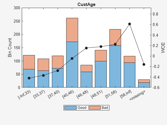

Display bin information for categorical data for 'ResStatus' that includes missing data in a separate bin labelled <missing>.

[bi,cg] = bininfo(sc,'ResStatus');
disp(bi)

         Bin          Good    Bad     Odds        WOE       InfoValue 
    ______________    ____    ___    ______    _________    __________

    {'Tenant'    }    296     161    1.8385    -0.095463     0.0035249
    {'Home Owner'}    352     171    2.0585     0.017549    0.00013382
    {'Other'     }    128      52    2.4615      0.19637     0.0055808
    {'<missing>' }     27      13    2.0769     0.026469    2.3248e-05
    {'Totals'    }    803     397    2.0227          NaN     0.0092627

disp(cg)

       Category       BinNumber
    ______________    _________

    {'Tenant'    }        1    
    {'Home Owner'}        2    
    {'Other'     }        3    

Note that the category grouping table does not include <missing> because this is a reserved bin and users cannot interact directly with the <missing> bin.

plotbins(sc,'ResStatus')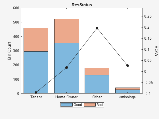

Input Arguments

sc — Credit scorecard model

creditscorecard object

Credit scorecard model, specified as a creditscorecard object. Use creditscorecard to create a creditscorecard object.

PredictorName — Predictor name

character vector

Predictor name, specified using a character vector containing the name of the predictor. PredictorName is case-sensitive.

Data Types: char

Name-Value Arguments

Specify optional pairs of arguments as Name1=Value1,...,NameN=ValueN, where Name is the argument name and Value is the corresponding value. Name-value arguments must appear after other arguments, but the order of the pairs does not matter.

Before R2021a, use commas to separate each name and value, and enclose Name in quotes.

Example: bi = bininfo(sc, PredictorName,'Statistics','WOE','Totals','On')

Statistics — List of statistics to include for bin information

{'Odds','WOE','InfoValue'} (default) | character vector with values 'Odds', 'WOE', 'InfoValue','Entropy', 'Gini', 'Chi2' | cell array of character vectors with values 'Odds', 'WOE', 'InfoValue', 'Entropy','Gini', 'Chi2'

List of statistics to include in the bin information, specified as the comma-separated pair consisting of 'Statistics' and a character vector or a cell array of character vectors. For more information, see Statistics for a Credit Scorecard. Possible values are:

• 'Odds' — Odds information is the ratio of “Goods” over “Bads.”

• 'WOE' — Weight of Evidence. The WOE Statistic measures the deviation between the distribution of “Goods” and “Bads.”

• 'InfoValue' — Information value. Closely tied to the WOE, it is a statistic used to determine how strong a predictor is to use in the fitting model. It measures how strong the deviation is between the distributions of “Goods” and “Bads.” However, bins with only “Good” or only “Bad” observations do lead to an infinite Information Value. Consider modifying the bins in those cases by using modifybins or autobinning.

• 'Entropy' — Entropy is a measure of unpredictability contained in the bins. The more the number of “Goods” and “Bads” differ within the bins, the lower the entropy.

• 'Gini' — Measure of statistical dispersion or inequality within a sample of data.

• 'Chi2' — Measure of statistical difference and independence between groups.

Note

Avoid having bins with frequencies of zero because they lead to infinite or undefined (NaN) statistics. Use modifybins or autobinning to modify bins.

Data Types: char | cell

Totals — Indicator to include row of totals at bottom information table

'On' (default) | character vector with values 'On', 'Off'

Indicator to include a row of totals at the bottom of the information table, specified as the comma-separated pair consisting of 'Totals' and a character vector with values On or Off.

Data Types: char

Output Arguments

bi — Bin information

table

Bin information, returned as a table. The bin information table contains one row per bin and a row of totals. The columns contain bin descriptions, frequencies of “Good” and “Bad,” and bin statistics. Avoid having bins with frequencies of zero because they lead to infinite or undefined (NaN) statistics. Use modifybins or autobinning to modify bins.

Note

When creating the creditscorecard object with creditscorecard, if the optional name-value pair argument WeightsVar was used to specify observation (sample) weights, then the bi table contains weighted counts.

bm — Binning map or rules

vector of cut points for numeric predictors | table of category groupings for categorical predictors

Binning map or rules, returned as a vector of cut points for numeric predictors, or a table of category groupings for categorical predictors. For more information, see modifybins.

mv — Binning minimum and maximum values

numeric array

Binning minimum and maximum values (as set or defined by the user), returned as a numeric array. The mv output argument is set to an empty array for categorical predictors.

More About

Statistics for a Credit Scorecard

Weight of Evidence (WOE) is a measure of the difference of the distribution of “Goods” and “Bads” within a bin.

Suppose the predictor's data takes on M possible values b1, ..., bM. For binned data, M is a small number. The response takes on two values, “Good” and “Bad.” The frequency table of the data is given by:

	Good	Bad	Total
b1:	n11	n12	n1
b2:	n21	n22	n2
bM:	nM1	nM2	nM
Total:	nGood	nBad	nTotal

The Weight of Evidence (WOE) is defined for each data value bi as

 WOE(i) = log((ni1/nGood)/(ni2/nBad)).

If you define

 pGood(i) = ni1/nGood, pBad(i) = ni2/nBad

then pGood(i) is the proportion of “Good” observations that take on the value bi, and similarly for pBad(i). In other words, pGood(i) gives the distribution of good observations over the M observed values of the predictor, and similarly for pBad(i). With this, an equivalent formula for the WOE is

WOE(i) = log(pGood(i)/pBad(i)).

Using the same frequency table, the odds for row i are defined as

Odds(i) = ni1 / ni2,

and the odds for the sample are defined as

OddsTotal = nGood / nBad.

For each row i, you can also compute its contribution to the total Information Value, given by

InfoValue(i) = (pGood(i) - pBad(i)) * WOE(i),

and the total Information Value is simply the sum of all the InfoValuel(i) terms. (A nansum is returned to discard contributions from rows with no observations at all.)

Likewise, for each row i, we can compute its contribution to the total Entropy, given by

 Entropy(i) = -1/log(2)*(ni1/ni*log(ni1/ni)+ni2/ni*log(ni2/ni),

and the total Entropy is simply the weighted sum of the row entropies,

Entropy = sum(ni/nTotal * Entropy(i)), i = 1...M.

Chi2 is computed pairwise for each pair of bins and measures the statistical difference between two groups when splitting or merging bins and is defined as:

 Chi2 = sum(sum((Aij - Eij)^2/Eij , j=1..k), i=m,m+1).

For more information on splitting and merging bins, see Split and Merge.

Gini ratio is a measure of the parent node, that is, of the given bins/categories prior to splitting or merging. The Gini ratio is defined as:

Gr = 1-G_hat/Gp

G_hat is the weighted Gini measure for the current split or merge:

G_hat = Sum((nj/N) * Gj, j=1..m).

For more information on splitting and merging bins, see Split and Merge.

Using bininfo with Weights

When observation weights are defined using the optional WeightsVar argument when creating a creditscorecard object, instead of counting the rows that are good or bad in each bin, the bininfo function accumulates the weight of the rows that are good or bad in each bin.

The “frequencies” reported are no longer the basic “count” of rows, but the “cumulative weight” of the rows that are good or bad and fall in a particular bin. Once these “weighted frequencies” are known, all other relevant statistics (Good, Bad, Odds, WOE, and InfoValue) are computed with the usual formulas. For more information, see Credit Scorecard Modeling Using Observation Weights.

References

[1] Anderson, R. The Credit Scoring Toolkit. Oxford University Press, 2007.

[2] Refaat, M. Credit Risk Scorecards: Development and Implementation Using SAS. lulu.com, 2011.

Version History

Introduced in R2014b