fevd
Generate forecast error variance decomposition (FEVD) of state-space model
Syntax
Description
The fevd function returns the forecast error variance decomposition (FEVD) of the measurement variables in a state-space model attributable to component-wise shocks to each state disturbance. The FEVD provides information about the relative importance of each state disturbance in affecting the forecast error variance of all measurement variables in the system. Other state-space model tools to characterize the dynamics of a specified system include the following:
The impulse response function (IRF), computed by
irfand plotted byirfplot, traces the effects of a shock to a state disturbance on the state and measurement variables in the system.Model-implied temporal correlations, computed by
corrfor a standard state-space model, measure the association between current and lagged state or measurement variables, as prescribed by the form of the model.
Fully Specified State-Space Model
Decomposition = fevd(Mdl)Decomposition of the fully specified state-space model Mdl.
Decomposition = fevd(Mdl,Name,Value)'NumPeriods',10 specifies estimating the FEVD for periods 1 through 10.
Partially Specified State-Space Model and Confidence Interval Estimation
Decomposition = fevd(___,'Params',estParams)Mdl. estParams specifies estimates of all unknown parameters in the model, using any of the input argument combinations in the previous syntaxes.
[ also returns the lower and upper 95% Monte Carlo confidence bounds Decomposition,Lower,Upper] = fevd(___,'Params',estParams,'EstParamCov',EstParamCov)Lower and Upper of each measurement variable FEVD. EstParamCov specifies the estimated covariance matrix of the parameter estimates, as returned by the estimate function, and is required for confidence interval estimation.
Examples
Compute the model-implied FEVD of two state-space models: one with measurement error and one without measurement error.
Model Without Measurement Error
Explicitly create the state-space model without measurement error
A = [1 0; 1 0.3];
B = [0.2 0; 0 1];
C = [1 0; 1 1];
Mdl1 = ssm(A,B,C,'StateType',[2 2])
Mdl1 =
State-space model type: ssm
State vector length: 2
Observation vector length: 2
State disturbance vector length: 2
Observation innovation vector length: 0
Sample size supported by model: Unlimited
State variables: x1, x2,...
State disturbances: u1, u2,...
Observation series: y1, y2,...
Observation innovations: e1, e2,...
State equations:
x1(t) = x1(t-1) + (0.20)u1(t)
x2(t) = x1(t-1) + (0.30)x2(t-1) + u2(t)
Observation equations:
y1(t) = x1(t)
y2(t) = x1(t) + x2(t)
Initial state distribution:
Initial state means
x1 x2
0 0
Initial state covariance matrix
x1 x2
x1 1e+07 0
x2 0 1e+07
State types
x1 x2
Diffuse Diffuse
Mdl1 is an ssm model object. Because all parameters have known values, the object is fully specified.
Compute the 20-period FEVD of the measurement variables.
Decomposition1 = fevd(Mdl1);
size(Decomposition1)
ans = 1×3

    20     2     2
Decomposition is a 20-by-2-by-2 array representing the 20-period FEVD of the two measurement variables. Display Decomposition(5,1,2).
Decomposition1(5,1,2)
ans =
0.4429
In this case, 44.29% of the volatility of is attributed to the shock applied to .
Plot the FEVD of for each state disturbance.
bar(Decomposition1(:,:,2),'stacked')
xlabel('Period')
ylabel('Variance Decompositions of $y_{2,t}$','Interpreter','latex')
legend('$u_{1,t}$','$u_{2,t}$','Interpreter','latex')
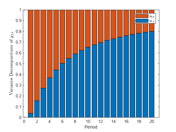
Because the state-space model is free of measurement error ( = 0), the variance decompositions of each period sum to 1. The volatility attributable to increases with each period.
Model with Measurement Error
Explicitly create the state-space model
D = eye(2);
Mdl2 = ssm(A,B,C,D,'StateType',[2 2])
Mdl2 =
State-space model type: ssm
State vector length: 2
Observation vector length: 2
State disturbance vector length: 2
Observation innovation vector length: 2
Sample size supported by model: Unlimited
State variables: x1, x2,...
State disturbances: u1, u2,...
Observation series: y1, y2,...
Observation innovations: e1, e2,...
State equations:
x1(t) = x1(t-1) + (0.20)u1(t)
x2(t) = x1(t-1) + (0.30)x2(t-1) + u2(t)
Observation equations:
y1(t) = x1(t) + e1(t)
y2(t) = x1(t) + x2(t) + e2(t)
Initial state distribution:
Initial state means
x1 x2
0 0
Initial state covariance matrix
x1 x2
x1 1e+07 0
x2 0 1e+07
State types
x1 x2
Diffuse Diffuse
Compute the 20-period FEVD of the measurement variables.
Decomposition2 = fevd(Mdl2);
Plot the FEVD of for each state disturbance.
bar(Decomposition2(:,:,2),'stacked')
xlabel('Period')
ylabel('Variance Decompositions of $y_{2,t}$','Interpreter','latex')
legend('$u_{1,t}$','$u_{2,t}$','Interpreter','latex')
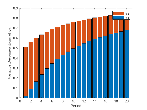
Because the model contains measurement error, the variance proportions do not sum to 1 during each period.
Explicitly create the multivariate diffuse state-space model
A = [1 0; 1 0.3];
B = [0.2 0; 0 1];
C = [1 0; 1 1];
Mdl = dssm(A,B,C,'StateType',[2 2])
Mdl =
State-space model type: dssm
State vector length: 2
Observation vector length: 2
State disturbance vector length: 2
Observation innovation vector length: 0
Sample size supported by model: Unlimited
State variables: x1, x2,...
State disturbances: u1, u2,...
Observation series: y1, y2,...
Observation innovations: e1, e2,...
State equations:
x1(t) = x1(t-1) + (0.20)u1(t)
x2(t) = x1(t-1) + (0.30)x2(t-1) + u2(t)
Observation equations:
y1(t) = x1(t)
y2(t) = x1(t) + x2(t)
Initial state distribution:
Initial state means
x1 x2
0 0
Initial state covariance matrix
x1 x2
x1 Inf 0
x2 0 Inf
State types
x1 x2
Diffuse Diffuse
Mdl is a dssm model object.
Compute the 50-period FEVD of the measurement variables.
Decomposition = fevd(Mdl,'NumPeriods',50);
size(Decomposition)
ans = 1×3
50 2 2
Plot the FEVD of for each state disturbance.
bar(Decomposition(:,:,2),'stacked')
xlabel('Period')
ylabel('Variance Decompositions of $y_{2,t}$','Interpreter','latex')
legend('$u_{1,t}$','$u_{2,t}$','Interpreter','latex')
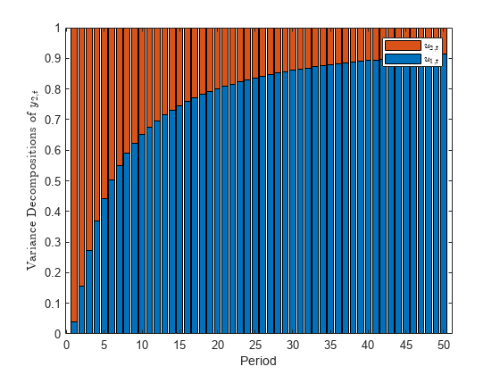
The contribution of to the volatility of approaches 90%.
Simulate data from a known model, fit the data to a state-space model, and then estimate the FEVD of the measurement variables.
Consider the time series decomposition , where is a random walk with drift representing the trend component, and is an AR(1) model representing the cycle component.
The model in state-space notation is
where is a dummy state representing the drift parameter, which is 1 for all .
Simulate 500 observations from the true model.
rng(1); % For reproducibility
ADGP = [1 3 0; 0 1 0; 0 0 0.5];
BDGP = [1 0; 0 0; 0 2];
CDGP = [1 0 1];
DGP = ssm(ADGP,BDGP,CDGP,'StateType',[2 1 0]);
y = simulate(DGP,500);
Assume that the drift constant, disturbance variances, and AR coefficient are unknown. Explicitly create a state-space model template for estimation that represents the model by replacing the unknown parameters in the model with NaN.
A = [1 NaN 0; 0 1 0; 0 0 NaN];
B = [NaN 0; 0 0; 0 NaN];
C = CDGP;
Mdl = ssm(A,B,C,'StateType',[2 1 0]);
Fit the model template to the data. Specify a set of positive, random standard Gaussian starting values for the four model parameters. Return the estimated model and vector of parameter estimates.
[EstMdl,estParams] = estimate(Mdl,y,abs(randn(4,1)),'Display','off')
EstMdl =
State-space model type: ssm

State vector length: 3
Observation vector length: 1
State disturbance vector length: 2
Observation innovation vector length: 0
Sample size supported by model: Unlimited

State variables: x1, x2,...
State disturbances: u1, u2,...
Observation series: y1, y2,...
Observation innovations: e1, e2,...

State equations:
x1(t) = x1(t-1) + (2.91)x2(t-1) + (0.92)u1(t)
x2(t) = x2(t-1)
x3(t) = (0.52)x3(t-1) + (2.13)u2(t)

Observation equation:
y1(t) = x1(t) + x3(t)

Initial state distribution:

Initial state means
 x1  x2  x3
  0   1   0

Initial state covariance matrix
     x1        x2  x3
 x1  1.00e+07   0   0
 x2   0         0   0
 x3   0         0  6.20

State types
    x1       x2         x3
 Diffuse  Constant  Stationary
estParams = 4×1

    2.9115
    0.5189
    0.9201
    2.1278
EstMdl is a fully specified ssm model object. Model estimates are close to their true values.
Compute and plot the FEVD of the measurement variable. Specify the model template Mdl and the vector of estimated parameters estParams.
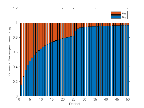
Decomposition = fevd(Mdl,'Params',estParams);

bar(Decomposition,'stacked')
xlabel('Period')
ylabel('Variance Decompositions of $y_{t}$','Interpreter','latex')
legend('$u_{1,t}$','$u_{2,t}$','Interpreter','latex')
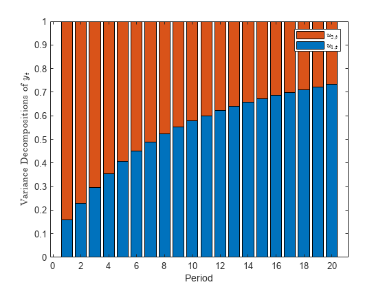
Noise in the cyclical component dominates the volatility of the measurement variable in low lags, with increasing contribution from the trend component noise as the lag increases.
Simulate data from a time-varying state-space model, fit a model to the data, and then estimate the time-varying FEVD of the measurement variable.
Consider the time series decomposition , where is a random walk with drift representing the trend component, and is an AR(1) model representing the cyclical component. Suppose that the cyclical component changes during period 26 over a 50-period time span.
Write a function that specifies how the parameters params map to the state-space model matrices, the initial state moments, and the state types. Save this code as a file named timeVariantTrendCycleParamMap.m on your MATLAB® path. Alternatively, open the example to access the function.
type timeVariantTrendCycleParamMap.m% Copyright 2021 The MathWorks, Inc.
function [A,B,C,D,Mean0,Cov0,StateType] = timeVariantTrendCycleParamMap(params)
% Time-varying state-space model parameter mapping function example. This
% function maps the vector params to the state-space matrices (A, B, C, and
% D). The measurement equation is a times series decomposed into trend and
% cyclical components, with a structural break in the cycle during period
% 26.
%
% The trend component is tau_t = drift + tau_{t-1} + s_1u1_t.
%
% The cyclical component is:
% * c_t = phi_1*c_{t-1} + s_2*u2_t; t = 1 through 25
% * c_t = phi_2*c_{t-1} + s_3*u2_t; t = 11 through 26.
%
% The measurement equation is y_t = tau_t + c_t.
A1 = {[1 params(1) 0; 0 1 0; 0 0 params(2)]};
A2 = {[1 params(1) 0; 0 1 0; 0 0 params(3)]};
varu1 = exp(params(4)); % Positive variance constraints
varu21 = exp(params(5));
varu22 = exp(params(6));
B1 = {[sqrt(varu1) 0; 0 0; 0 sqrt(varu21)]};
B2 = {[sqrt(varu1) 0; 0 0; 0 sqrt(varu22)]};
C = [1 0 1];
D = 0;
sc = 25;
A = [repmat(A1,sc,1); repmat(A2,sc,1)];
B = [repmat(B1,sc,1); repmat(B2,sc,1)];
Mean0 = [];
Cov0 = [];
StateType = [2 1 0];
end
Implicitly create a partially specified state-space model representing the data generating process (DGP).
ParamMap = @timeVariantTrendCycleParamMap;
DGP = ssm(ParamMap);
Simulate 50 observations from the DGP. Because DGP is partially specified, pass the true parameter values to simulate by using the 'Params' name-value argument.
rng(5) % For reproducibility
trueParams = [1 0.5 -0.2 2*log(1) 2*log(2) 2*log(0.5)]; % Transform variances for parameter map
y = simulate(DGP,50,'Params',trueParams);
y is a 50-by-1 vector of simulated measurements from the DGP.
Because DGP is a partially specified, implicit model object, its parameters are unknown. Therefore, it can serve as a model template for estimation.
Fit the model to the simulated data. Specify random standard Gaussian draws for the initial parameter values, and turn off the estimation display. Return the parameter estimates.
[~,estParams] = estimate(DGP,y,randn(1,6),'Display','off')
estParams = 1×6

    0.8510    0.0137    0.6316   -0.3253    1.3793   -0.2179
estParams is a 1-by-6 vector of parameter estimates. The output argument list of the parameter mapping function determines the order of the estimates.
Estimate the FEVD of the measurement variable by supplying DGP (not the estimated model) and the estimated parameters using the 'Params' name-value argument.
Decomposition = fevd(DGP,'Params',estParams,'NumPeriods',50);

bar(Decomposition,'stacked')
xlabel('Period')
ylabel('Variance Decompositions of $y_{t}$','Interpreter','latex')
legend('$u_{1,t}$','$u_{2,t}$','Interpreter','latex')
The FEVD jumps at period 26, when the structural break occurs.
Simulate data from a known model, fit the data to a state-space model, and then estimate the FEVD of the measurement variables with 90% Monte Carlo confidence bounds.
Consider the time series decomposition , where is a random walk with drift representing the trend component, and is an AR(1) model representing the cycle component.
The model in state-space notation is
where is a dummy state representing the drift parameter, which is 1 for all t.
Simulate 500 observations from the true model.
rng(1); % For reproducibility
ADGP = [1 3 0; 0 1 0; 0 0 0.5];
BDGP = [1 0; 0 0; 0 2];
CDGP = [1 0 1];
DGP = ssm(ADGP,BDGP,CDGP,'StateType',[2 1 0]);
y = simulate(DGP,500);
Assume that the drift constant, disturbance variances, and AR coefficient are unknown. Explicitly create a state-space model template for estimation that represents the model by replacing the unknown parameters in the model with NaN.
A = [1 NaN 0; 0 1 0; 0 0 NaN];
B = [NaN 0; 0 0; 0 NaN];
C = CDGP;
Mdl = ssm(A,B,C,'StateType',[2 1 0]);
Fit the model template to the data. Specify a set of positive, random standard Gaussian starting values for the four model parameters, and turn off the estimation display. Return the estimated model and vector of parameter estimates and their estimated covariance matrix.
[EstMdl,estParams,EstParamCov] = estimate(Mdl,y,abs(randn(4,1)),'Display','off');
EstMdl is a fully specified ssm model object. Model estimates are close to their true values.
Compute the FEVD of the measurement variable with period-wise 90% Monte Carlo confidence bounds. Specify the model template Mdl, vector of estimated parameters estParams, and their estimated covariance matrix EstParamCov.
[Decomposition,Lower,Upper] = fevd(Mdl,'Params',estParams,'EstParamCov',EstParamCov,...
    'Confidence',0.9);
Plot the proportion of volatility of attributable to with corresponding 90% confidence bounds.
plot(Decomposition(:,1),'r-o')
hold on
plot([Lower(:,1) Upper(:,1)],'b-o')
hold off
xlabel('Period')
ylabel('Proportion of Volatility')
title('Volatility Attributable to $u_{1,t}$','Interpreter','latex')
legend('Proportion','90% confidence bounds')
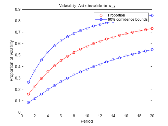
The confidence bounds are initially relatively tight, but widen as the lag and volatility increase.
Input Arguments
Name-Value Arguments
Output Arguments
More About
Algorithms
If you do not supply the
EstParamCovname-value argument, confidence bounds of each period overlap.fevduses Monte Carlo simulation to compute confidence intervals.fevdrandomly drawsNumPathsvariates from the asymptotic sampling distribution of the unknown parameters inMdl, which is Np(Params,EstParamCov), where p is the number of unknown parameters.For each randomly drawn parameter set j,
fevddoes the following:Create a state-space model that is equal to
Mdl, but substitute in parameter set j.Compute the random FEVD of the resulting model γj(t), where t = 1 through
NumPaths.
For each time t, the lower bound of the confidence interval is the
(1 –quantile of the simulated FEVD at period t γ(t), wherec)/2cConfidence. Similarly, the upper bound of the confidence interval at time t is the(1 –upper quantile of γ(t).c)/2
Version History
Introduced in R2021a