infer

Infer residuals of univariate regression model with ARIMA time series errors

Syntax

E = infer(Mdl,Y)

[E,U,V] = infer(Mdl,Y)

Tbl2 = infer(Mdl,Tbl1)

[___] = infer(___,Name=Value)

[___,logL] = infer(___)

Description

E = infer(Mdl,Y) returns the numeric array of one or more residual series E inferred from the fully specified, univariate regression model with ARIMA time series errors Mdl and the numeric array of one or more response series Y.

[E,U,V] = infer(Mdl,Y) also returns the numeric array of one or more unconditional disturbance U and innovation variance V series.

Tbl2 = infer(Mdl,Tbl1) returns the table or timetable Tbl2 containing paths of residuals, unconditional disturbances, innovation variances inferred from the model Mdl and the response data in the input table or timetable Tbl1. (since R2023b)

infer selects the response variable named in Mdl.SeriesName or the sole variable in Tbl1. To select a different response variable in Tbl1 to infer residuals, unconditional disturbances, and innovation variances, use the ResponseVariable name-value argument.

[___] = infer(___,Name=Value) specifies options using one or more name-value arguments in addition to any of the input argument combinations in previous syntaxes. infer returns the output argument combination for the corresponding input arguments. For example, infer(Mdl,Y,U0=u0,X=Pred) infers residuals from the numeric vector of response data Y with respect to the regression model with ARIMA errors Mdl, and specifies the numeric vector of presample regression model residual data u0 to initialize the model and the predictor data Pred for the regression component.

[___,logL] = infer(___) also returns a numeric vector containing the loglikelihood objective function values logL associated with each specified path of response data.

Examples

Infer Vector of Residuals from Regression Model with ARIMA Errors

Infer error model residuals from a simulated path of responses from the following regression model with ARMA(2,1) errors:

$$\begin{array}{l}\begin{array}{c}{y}_t=X_t\left[\begin{array}{c}0.1\\ -0.2\end{array}\right]+u_t\\ u_t=0.5u_{t-1}-0.8u_{t-2}+{\epsilon }_t-0.5{\epsilon }_{t-1},\end{array}\end{array}$$

where $${\epsilon }_t$$ is Gaussian with variance 0.1. Assume the predictors are standard Gaussian random variables. Provide data as numeric arrays.

Create the regression model with ARIMA errors. Simulate responses from the model and two predictor series.

Mdl = regARIMA(Intercept=0,AR={0.5 -0.8},MA=-0.5, ...
    Beta=[0.1; -0.2],Variance=0.1);

rng(1,"twister"); % For reproducibility
Pred = randn(100,2);
y = simulate(Mdl,100,X=Pred);

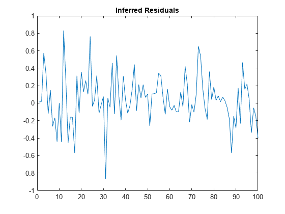
Infer and plot the error model residuals. By default, infer backcasts for the necessary presample unconditional disturbances and sets necessary presample error model residuals to zero.

e = infer(Mdl,y,X=Pred);

figure
plot(e)
title("Inferred Residuals")

e is a 100-by-1 vector of error model residuals, associated with error model innovations ${\epsilon }_{\mathit{t}}$.

Examine Residuals of Estimated Model in Timetable

Since R2023b

Fit a regression model with ARMA(1,1) errors by regressing the US gross domestic product (GDP) growth rate onto consumer price index (CPI) quarterly changes. Examine the error model and regression residuals. Supply a timetable of data and specify the series for the fit.

Load and Transform Data

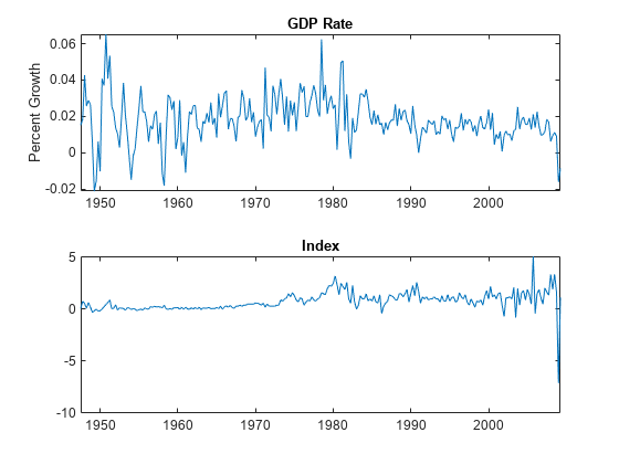
Load the US macroeconomic data set. Compute the series of GDP quarterly growth rates and CPI quarterly changes.

load Data_USEconModel
DTT = price2ret(DataTimeTable,DataVariables="GDP");
DTT.GDPRate = 100*DTT.GDP;
DTT.CPIDel = diff(DataTimeTable.CPIAUCSL);
T = height(DTT) 

T = 
248

figure
tiledlayout(2,1)
nexttile
plot(DTT.Time,DTT.GDPRate)
title("GDP Rate")
ylabel("Percent Growth")
nexttile
plot(DTT.Time,DTT.CPIDel)
title("Index")

The series appear stationary, albeit heteroscedastic.

Prepare Timetable for Estimation

When you plan to supply a timetable, you must ensure it has all the following characteristics:

• The selected response variable is numeric and does not contain any missing values.

• The timestamps in the Time variable are regular, and they are ascending or descending.

Remove all missing values from the timetable.

DTT = rmmissing(DTT);
T_DTT = height(DTT)

T_DTT = 
248

Because each sample time has an observation for all variables, rmmissing does not remove any observations.

Determine whether the sampling timestamps have a regular frequency and are sorted.

areTimestampsRegular = isregular(DTT,"quarters")

areTimestampsRegular = logical
   0

areTimestampsSorted = issorted(DTT.Time)

areTimestampsSorted = logical
   1

areTimestampsRegular = 0 indicates that the timestamps of DTT are irregular. areTimestampsSorted = 1 indicates that the timestamps are sorted. Macroeconomic series in this example are timestamped at the end of the month. This quality induces an irregularly measured series.

Remedy the time irregularity by shifting all dates to the first day of the quarter.

dt = DTT.Time;
dt = dateshift(dt,"start","quarter");
DTT.Time = dt;
areTimestampsRegular = isregular(DTT,"quarters")

areTimestampsRegular = logical
   1

DTT is regular.

Create Model Template for Estimation

Suppose that a regression model of CPI quarterly changes onto the GDP rate, with ARMA(1,1) errors, is appropriate.

Create a model template for a regression model with ARMA(1,1) errors template. Specify the response variable name.

Mdl = regARIMA(1,0,1);
Mdl.SeriesName = "GDPRate";

Mdl is a partially specified regARIMA object.

Fit Model to Data

Fit a regression model with ARMA(1,1) errors to the data. Specify the entire series GDP rate and CPI quarterly changes series, and specify the predictor variable name.

EstMdl = estimate(Mdl,DTT,PredictorVariables="CPIDel");

 
    Regression with ARMA(1,1) Error Model (Gaussian Distribution):
 
                  Value      StandardError    TStatistic      PValue  
                 ________    _____________    __________    __________

    Intercept      0.0162      0.0016077        10.077      6.9994e-24
    AR{1}         0.60515       0.089912        6.7305      1.6906e-11
    MA{1}        -0.16221        0.11051       -1.4678         0.14216
    Beta(1)      0.002221     0.00077691        2.8587       0.0042532
    Variance     0.000113     7.2753e-06        15.533      2.0838e-54

EstMdl is a fully specified, estimated regARIMA object. By default, estimate backcasts for the required Mdl.P = 1 presample regression model residual and sets the required Mdl.Q = 1 presample error model residual to 0.

Examine Residuals

Infer a timetable of error model and regression residuals for all observations. Specify the predictor variable name.

Tbl2 = infer(EstMdl,DTT,PredictorVariables="CPIDel")

Tbl2=248×6 timetable
    Time     Interval        GDP         GDPRate     CPIDel    GDPRate_ErrorResidual    GDPRate_RegressionResidual
    _____    ________    ___________    _________    ______    _____________________    __________________________

    Q2-47       91        0.00015183     0.015183     0.08          -0.0007572                  -0.0011947        
    Q3-47       92        0.00018374     0.018374     0.76           0.0010863                  0.00048617        
    Q4-47       92          0.000427       0.0427     0.57            0.025116                    0.025234        
    Q1-48       91        0.00025617     0.025617     0.09          -0.0019795                   0.0092168        
    Q2-48       91        0.00028739     0.028739     0.65            0.005197                    0.011096        
    Q3-48       92        0.00026512     0.026512     0.21           0.0039745                   0.0098461        
    Q4-48       92        5.1468e-05    0.0051468    -0.31           -0.015678                   -0.010365        
    Q1-49       90       -0.00021196    -0.021196    -0.14           -0.033356                   -0.037085        
    Q2-49       91       -0.00015576    -0.015576     0.01           -0.014767                   -0.031798        
    Q3-49       92        6.1077e-05    0.0061077    -0.17           0.0071327                  -0.0097147        
    Q4-49       91       -0.00010311    -0.010311    -0.14           -0.019164                     -0.0262        
    Q1-50       91        0.00040675     0.040675     0.03            0.037154                    0.024408        
    Q2-50       91        0.00036908     0.036908     0.24            0.011432                    0.020175        
    Q3-50       91        0.00065211     0.065211     0.46            0.037635                     0.04799        
    Q4-50       91        0.00040718     0.040718     0.64          0.00016008                    0.023097        
    Q1-51       91        0.00053382     0.053382      0.9            0.021232                    0.035183        
      ⋮

Tbl2 is a 248-by-6 timetable containing the error model residuals GDPRate_ErrorResidual, regression residuals GDPRate_RegressionResidual, and all variables in DTT.

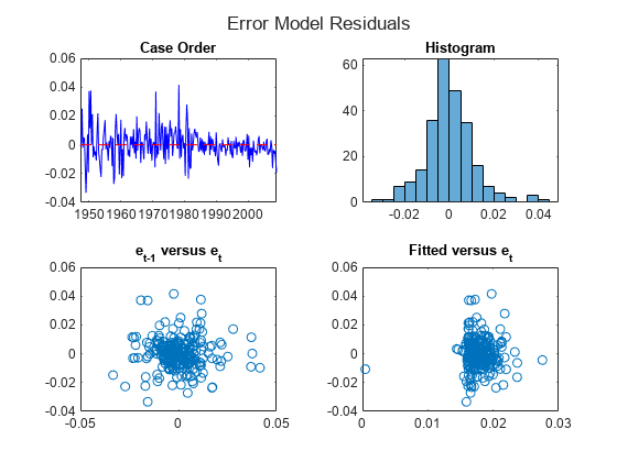
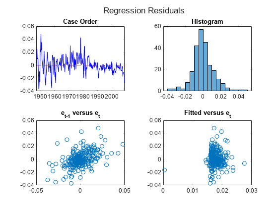
Separately plot the inferred error model and regression residuals.

Tbl2.GDPRate_Fitted = Tbl2.GDPRate - Tbl2.GDPRate_RegressionResidual;

figure
h = tiledlayout(2,2);
title(h,"Error Model Residuals")
nexttile
plot(Tbl2.Time,Tbl2.GDPRate_ErrorResidual,'b',Tbl2.Time([1 end]),[0 0],'--r')
title("Case Order")
nexttile
histogram(Tbl2.GDPRate_ErrorResidual)
title("Histogram")
nexttile
plot(Tbl2.GDPRate_ErrorResidual(1:end-1),Tbl2.GDPRate_ErrorResidual(2:end),'o')
title("e_{t-1} versus e_t")
nexttile
plot(Tbl2.GDPRate_Fitted,Tbl2.GDPRate_ErrorResidual,'o')
title("Fitted versus e_t")

figure
h = tiledlayout(2,2);
title(h,"Regression Residuals")
nexttile
plot(Tbl2.Time,Tbl2.GDPRate_RegressionResidual,'b',Tbl2.Time([1 end]),[0 0],'--r')
title("Case Order")
nexttile
histogram(Tbl2.GDPRate_RegressionResidual)
title("Histogram")
nexttile
plot(Tbl2.GDPRate_RegressionResidual(1:end-1),Tbl2.GDPRate_RegressionResidual(2:end),'o')
title("e_{t-1} versus e_t")
nexttile
plot(Tbl2.GDPRate_Fitted,Tbl2.GDPRate_RegressionResidual,'o')
title("Fitted versus e_t")

Compare Model Fits By Using Likelihood Ratio Test

Fit this regression model with ARMA(2,1) errors to simulated data:

$$\begin{array}{l}\begin{array}{c}{y}_t=1+X_t\left[\begin{array}{c}0.1\\ -0.2\end{array}\right]+u_t\\ u_t=0.5u_{t-1}-0.8u_{t-2}+{\epsilon }_t-0.5{\epsilon }_{t-1},\end{array}\end{array}$$

where $${\epsilon }_t$$ is Gaussian with variance 0.1. Compare the fit to an intercept-only regression model by conducting a likelihood ratio test. Provide response and predictor data in vectors.

Simulate Data

Specify the regression model ARMA(2,1) errors. Simulate responses from the model, and simulate two predictor series from the standard Gaussian distribution.

Mdl0 = regARIMA(Intercept=1,AR={0.5 -0.8},MA=-0.5, ...
    Beta=[0.1; -0.2],Variance=0.1);

rng(1,"twister")  % For reproducibility
Pred =  randn(100,2);
y = simulate(Mdl0,100,X=Pred);

y is a 100-by-1 random response path simulated from Mdl.

Fit Unrestricted Model

Create an unrestricted model template of a regression model with ARMA(2,1) errors for estimation.

Mdl = regARIMA(2,0,1)

Mdl = 
  regARIMA with properties:

     Description: "ARMA(2,1) Error Model (Gaussian Distribution)"
      SeriesName: "Y"
    Distribution: Name = "Gaussian"
       Intercept: NaN
            Beta: [1×0]
               P: 2
               Q: 1
              AR: {NaN NaN} at lags [1 2]
             SAR: {}
              MA: {NaN} at lag [1]
             SMA: {}
        Variance: NaN

The AR coefficients, MA coefficients, and the innovation variance are NaN values. estimate estimates those parameters. When Beta is an empty array, estimate determines the number of regression coefficients to estimate.

Fit the unrestricted model to the data. Specify the predictor data.

EstMdlUR = estimate(Mdl,y,X=Pred);

 
    Regression with ARMA(2,1) Error Model (Gaussian Distribution):
 
                  Value      StandardError    TStatistic      PValue  
                 ________    _____________    __________    __________

    Intercept      1.0167      0.010154         100.13               0
    AR{1}         0.64995      0.093794         6.9295      4.2226e-12
    AR{2}        -0.69174      0.082575        -8.3771      5.4247e-17
    MA{1}        -0.64508       0.11055         -5.835      5.3796e-09
    Beta(1)       0.10866      0.020965          5.183      2.1835e-07
    Beta(2)      -0.20979      0.022824        -9.1917      3.8679e-20
    Variance     0.073117      0.008716         8.3888      4.9121e-17

EstMdlUR is a fully specified regARIMA object representing the estimated unrestricted regression model with ARIMA errors.

Fit Restricted Model

The restricted model contains the same error model, but the regression model contains only an intercept. That is, the restricted model imposes two restrictions on the unrestricted model: ${\beta }_1={\beta }_2=0$.

Fit the restricted model to the data.

EstMdlR = estimate(Mdl,y);

 
    ARMA(2,1) Error Model (Gaussian Distribution):
 
                  Value      StandardError    TStatistic      PValue  
                 ________    _____________    __________    __________

    Intercept      1.0176      0.024905         40.859               0
    AR{1}         0.51541       0.18536         2.7805       0.0054271
    AR{2}        -0.53359       0.10949        -4.8735      1.0963e-06
    MA{1}        -0.34923       0.19423         -1.798         0.07218
    Variance       0.1445      0.020214         7.1486      8.7671e-13

EstMdlR is a fully specified regARIMA object representing the estimated restricted regression model with ARIMA errors.

Compute Residuals and Loglikelihoods

Compute the residual series and loglikelihoods for the estimated models.

[eUR,uUR,~,logLUR] = infer(EstMdlUR,y,X=Pred);
[eR,uR,~,logLR] = infer(EstMdlR,y);

eUR and uUR are 100-by-1 vectors containing the error model and regression residuals from the unrestricted estimation. loglUR is the corresponding loglikelihood.

eR and uR are 100-by-1 vectors containing the error model and regression residuals from the restricted estimation. loglR is the corresponding loglikelihood.

Conduct Likelihood Ratio Test

The likelihood ratio test requires the optimized loglikelihoods of the unrestricted and restricted models, and it requires the number of model restrictions (degrees of freedom).

Conduct a likelihood ratio test to determine which model has the better fit to the data.

dof = 2;
[h,p] = lratiotest(logLUR,logLR,dof)

h = logical
   1

p = 
1.6653e-15

The $\mathit{p}$-value is close to zero, which suggests that there is strong evidence to reject the null hypothesis that the data fits the restricted model better than the unrestricted model.

Input Arguments

Mdl — Fully specified regression model with ARIMA errors

regARIMA model object

Fully specified regression model with ARIMA errors, specified as a regARIMA model object created by regARIMA or estimate.

The properties of Mdl cannot contain NaN values.

Y — Response data y_t

numeric column vector | numeric matrix

Response data y_t, specified as a numobs-by-1 numeric column vector or numobs-by-numpaths numeric matrix. numObs is the length of the time series (sample size). numpaths is the number of separate, independent paths of response series.

infer infers the residuals, unconditional disturbances, and innovation variances of columns of Y, which are time series characterized by Mdl.

Each row corresponds to a sampling time. The last row contains the latest set of observations.

Each column corresponds to a separate, independent path of response data. infer assumes that responses across any row occur simultaneously.

Data Types: double

Tbl1 — Time series data

table | timetable

Since R2023b

Time series data containing the observed response variable y_t and, optionally, predictor variables x_t for the regression component, specified as a table or timetable with numvars variables and numobs rows. You can optionally select the response variable or numpreds predictor variables by using the ResponseVariable or PredictorVariables name-value arguments, respectively.

Each row is an observation, and measurements in each row occur simultaneously. The selected response variable is a single path (numobs-by-1 vector) or multiple paths (numobs-by-numpaths matrix) of numobs observations of response data.

Each path (column) of the selected response variable is independent of the other paths, but path j of all presample and in-sample variables correspond, for j = 1,…,numpaths. Each selected predictor variable is a numobs-by-1 numeric vector representing one path. The infer function includes all predictor variables in the model when it infers residuals. Variables in Tbl1 represent the continuation of corresponding variables in Presample.

If Tbl1 is a timetable, it must represent a sample with a regular datetime time step (see isregular), and the datetime vector Tbl1.Time must be strictly ascending or descending.

If Tbl1 is a table, the last row contains the latest observation.

Name-Value Arguments

Specify optional pairs of arguments as Name1=Value1,...,NameN=ValueN, where Name is the argument name and Value is the corresponding value. Name-value arguments must appear after other arguments, but the order of the pairs does not matter.

Before R2021a, use commas to separate each name and value, and enclose Name in quotes.

Example: infer(Mdl,Y,U0=u0,X=Pred) infers residuals from the numeric vector of response data Y with respect to the regression model with ARIMA errors Mdl, and specifies the numeric vector of presample regression model residual data u0 to initialize the model and the predictor data Pred for the regression component.

ResponseVariable — Response variable y_t to select from Tbl1

string scalar | character vector | integer | logical vector

Since R2023b

Response variable y_t to select from Tbl1 containing the response data, specified as one of the following data types:

• String scalar or character vector containing a variable name in Tbl1.Properties.VariableNames

• Variable index (positive integer) to select from Tbl1.Properties.VariableNames

• A logical vector, where DisturbanceVariable(j) = true selects variable j from Tbl1.Properties.VariableNames

The selected variable must be a numeric vector and cannot contain missing values (NaNs).

If Tbl1 has one variable, the default specifies that variable. Otherwise, the default matches the variable to names in Mdl.SeriesName.

Example: ResponseVariable="StockRate"

Example: ResponseVariable=[false false true false] or ResponseVariable=3 selects the third table variable as the response variable.

Data Types: double | logical | char | cell | string

X — Predictor data

numeric matrix

Predictor data for the model regression component, specified as a numeric matrix with numpreds columns. numpreds is the number of predictor variables (numel(Mdl.Beta)). Use X only when you supply the numeric array of response data Y.

X must have at least numobs rows. If the number of rows of X exceeds numobs, infer uses only the latest observations. infer does not use the regression component in the presample period.

Columns of X are separate predictor variables.

infer applies X to each path; that is, X represents one path of observed predictors.

By default, infer excludes the regression component, regardless of its presence in Mdl.

Data Types: double

PredictorVariables — Predictor variables x_t to select from Tbl1

string vector | cell vector of character vectors | vector of integers | logical vector

Predictor variables x_t to select from Tbl1 containing the predictor data for the model regression component, specified as one of the following data types:

• String vector or cell vector of character vectors containing numpreds variable names in Tbl1.Properties.VariableNames

• A vector of unique indices (positive integers) of variables to select from Tbl1.Properties.VariableNames

• A logical vector, where PredictorVariables(j) = true selects variable j from Tbl1.Properties.VariableNames

The selected variables must be numeric vectors and cannot contain missing values (NaNs).

By default, infer excludes the regression component, regardless of its presence in Mdl.

Example: PredictorVariables=["M1SL" "TB3MS" "UNRATE"]

Example: PredictorVariables=[true false true false] or PredictorVariable=[1 3] selects the first and third table variables to supply the predictor data.

Data Types: double | logical | char | cell | string

E0 — Presample error model residual data e_t

numeric column vector | numeric matrix

Presample error model residual data e_t to initialize the error model, specified as a numpreobs-by-1 numeric column vector or a numpreobs-by-numprepaths numeric matrix. Use E0 only when you supply the numeric array of response data Y.

Each row is a presample observation (sampling time), and measurements in each row occur simultaneously. The last row contains the latest presample observation. numpreobs must be at least Mdl.Q to initialize the moving average (MA) component of the error model. If numpreobs is larger than required, infer uses the latest required number of observations only.

Columns of E0 are separate, independent presample paths. The following conditions apply:

• If E0 is a column vector, it represents a single residual path. infer applies it to each output path.

• If E0 is a matrix, each column represents a presample residual path. infer applies E0(:,j) to initialize path j. numprepaths must be at least numpaths. If numprepaths > numpaths, infer uses the first size(Y,2) columns only.

• infer assumes each column of E0 has a mean of zero.

By default, infer sets the necessary presample disturbances to zero.

Data Types: double

U0 — Presample regression residual data

numeric column vector | numeric matrix

Presample regression residual data, associated with the unconditional disturbances u_t, to initialize the error model, specified as a numpreobs-by-1 numeric column vector or a numpreobs-by-numprepaths numeric matrix. Use U0 only when you supply the numeric array of response data Y.

Each row is a presample observation (sampling time), and measurements in each row occur simultaneously. The last row contains the latest presample observation. numpreobs must be at least Mdl.P to initialize the error model autoregressive (AR) component. If numpreobs is larger than required, infer uses the latest required observations only.

Columns of U0 are separate, independent presample paths. The following conditions apply:

• If U0 is a column vector, it represents a single path. infer applies it to each path.

• If U0 is a matrix, each column represents a presample path. infer applies U0(:,j) to initialize path j. numprepaths must be at least numpaths. If numprepaths > numpaths, infer uses the first size(Z,2) columns only.

By default, infer backcasts for necessary presample unconditional disturbances.

Data Types: double

Presample — Presample data

table | timetable

Since R2023b

Presample data containing paths of error model residual e_t or regression residual series to initialize the model, specified as a table or timetable, the same type as Tbl1, with numprevars variables and numpreobs rows. Regression residuals are associated with the unconditional disturbances u_t. Use Presample only when you supply a table or timetable of data Tbl1.

Each selected variable is a single path (numpreobs-by-1 vector) or multiple paths (numpreobs-by-numprepaths matrix) of numpreobs observations representing the presample of the error model or regression residual series for ResponseVariable, the selected response variable in Tbl1.

Each row is a presample observation, and measurements in each row occur simultaneously. numpreobs must be one of the following values:

• At least Mdl.P when Presample provides only presample regression residuals

• At least Mdl.Q when Presample provides only presample error model residuals

• At least max([Mdl.P Mdl.Q]) otherwise

If you supply more rows than necessary, infer uses the latest required number of observations only.

When Presample provides presample residuals, infer assumes each presample error model residual path has a mean of zero.

If Presample is a timetable, all the following conditions must be true:

• Presample must represent a sample with a regular datetime time step (see isregular).

• The inputs Tbl1 and Presample must be consistent in time such that Presample immediately precedes Tbl1 with respect to the sampling frequency and order.

• The datetime vector of sample timestamps Presample.Time must be ascending or descending.

If Presample is a table, the last row contains the latest presample observation.

By default, infer backcasts for necessary presample regression residuals and sets necessary presample error model residuals to zero.

If you specify the Presample, you must specify the presample error model or regression residual name by using the PresampleInnovationVariable or PresampleRegressionDisturbanceVariable name-value argument.

PresampleInnovationVariable — Error model residual e_t to select from Presample

string scalar | character vector | integer | logical vector

Since R2023b

Error model residual variable e_t to select from Presample containing the presample error model residual data, specified as one of the following data types:

• String scalar or character vector containing the variable name to select from Presample.Properties.VariableNames

• Variable index (positive integer) to select from Presample.Properties.VariableNames

• A logical vector, where PresampleInnovationVariable(j) = true selects variable j from Presample.Properties.VariableNames

The selected variable must be a numeric vector and cannot contain missing values (NaNs).

If you specify presample error model residual data by using the Presample name-value argument, you must specify PresampleInnovationVariable.

Example: PresampleInnovationVariable="GDP_Z"

Example: PresampleInnovationVariable=[false false true false] or PresampleInnovationVariable=3 selects the third table variable for presample error model residual data.

Data Types: double | logical | char | cell | string

PresampleRegressionDistrubanceVariable — Regression model residual variable to select from Presample

string scalar | character vector | integer | logical vector

Since R2023b

Regression model residual variable, associated with unconditional disturbances u_t, to select from Presample containing data for the presample regression model residuals, specified as one of the following data types:

• String scalar or character vector containing a variable name in Presample.Properties.VariableNames

• Variable index (positive integer) to select from Presample.Properties.VariableNames

• A logical vector, where PresampleRegressionDistrubanceVariable(j) = true selects variable j from Presample.Properties.VariableNames

The selected variable must be a numeric vector and cannot contain missing values (NaNs).

If you specify presample regression model residual data by using the Presample name-value argument, you must specify PresampleRegressionDistrubanceVariable.

Example: PresampleRegressionDistrubanceVariable="StockRateU"

Example: PresampleRegressionDistrubanceVariable=[false false true false] or PresampleRegressionDistrubanceVariable=3 selects the third table variable as the presample regression model residual data.

Data Types: double | logical | char | cell | string

Note

• NaN values in Y, X, E0 and U0 indicate missing values. infer removes missing values from specified data by listwise deletion.

  • For the presample, infer horizontally concatenates the possibly jagged arrays E0 and U0 with respect to the last rows, and then it removes any row of the concatenated matrix containing at least one NaN.

  • For in-sample data, infer horizontally concatenates the possibly jagged arrays Y and X, and then it removes any row of the concatenated matrix containing at least one NaN.

  This type of data reduction reduces the effective sample size and can create an irregular time series.

• For numeric data inputs, infer assumes that you synchronize the presample data such that the latest observations occur simultaneously.

• infer issues an error when any table or timetable input contains missing values.

• All predictor variables (columns) in X are associated with each input response series to produce numpaths output series.

Output Arguments

E — Inferred error model residuals e_t

numeric matrix

Inferred error model residuals e_t, returned as a numobs-by-numpaths numeric matrix. infer returns E only when you supply the input Y.

E(j,k) is the path k error model residual of time j; it is the error model residual associated with response Y(j,k).

Inferred residuals are

$$e_t={\widehat{u}}_t-{\varphi }_1{\widehat{u}}_{t-1}-\mathrm{...}-{\varphi }_P{\widehat{u}}_{t-P}-{\theta }_1{e}_{t-1}-\mathrm{...}-{\theta }_Q{e}_{t-Q}$$

$${\widehat{u}}_t$$ is row t of the inferred unconditional disturbances U, ϕ_j is composite autoregressive coefficient j, and θ_k is composite moving average coefficient k.

U — Inferred regression residuals

numeric matrix

Inferred regression residuals associated with the unconditional disturbances u_t, returned as a numobs-by-numpaths numeric matrix. infer returns V only when you supply the input Y.

U(j,k) is the path k regression model residual of time j; it is the regression model residual associated with response Y(j,k).

Inferred unconditional disturbances are

$${\widehat{u}}_t=y_t-c-x_t\beta .$$

y_t is row t of the response data Y, x_t is row t of the predictor data X, c is the model intercept Mdl.Intercept, and β is the vector of regression coefficients Mdl.Beta.

V — Inferred innovation variances

numeric matrix

Inferred innovation variances, returned as a numobs-by-numpaths numeric matrix. infer returns V only when you supply the input Y. All elements in V are equal to Mdl.Variance.

Tbl2 — Inferred error model residual e_t and regression residual paths

table | timetable

Since R2023b

Inferred error model residual e_t and regression residual paths, returned as a table or timetable, the same data type as Tbl1. infer returns Tbl2 only when you supply the input Tbl1. Regression residuals are associated with the unconditional disturbances u_t.

Tbl2 contains the following variables:

• The inferred error model residual paths, which are in a numobs-by-numpaths numeric matrix, with rows representing observations and columns representing independent paths. Each path corresponds to the input response path in Tbl1 and represents the continuation of the corresponding presample error model residual path in Presample. infer names the inferred residual variable in Tbl2 responseName_ErrorResidual, where responseName is Mdl.SeriesName. For example, if Mdl.SeriesName is StockReturns, Tbl2 contains a variable for the corresponding inferred error model residual paths with the name StockReturns_ErrorResidual.

• The inferred regression residual paths, which are in a numobs-by-numpaths numeric matrix, with rows representing observations and columns representing independent paths. Each path represents the continuation of the corresponding path of presample regression residuals in Presample. infer names the inferred regression residual variable in Tbl2 responseName_RegressionResidual, where responseName is Mdl.SeriesName. For example, if Mdl.SeriesName is StockReturns, Tbl2 contains a variable for the corresponding inferred regression residual paths with the name StockReturns_RegressionResidual.

• All variables Tbl1.

If Tbl1 is a timetable, row times of Tbl1 and Tbl2 are equal.

Tbl2 does not include a variable containing inferred paths of innovation variances. To create such a variable, enter Tbl2.responseName_Variance = Mdl.Variance*ones(size(Tbl2));.

logL — Loglikelihood objective function values

numeric scalar | numeric vector

Loglikelihood objective function values associated with the model Mdl, returned as a numeric scalar or vector of length numpaths.

If Y is a vector, then logL is a scalar. Otherwise, logL is vector of length size(Y,2), and each element is the loglikelihood of the corresponding column (or path) in Y.

References

[1] Box, George E. P., Gwilym M. Jenkins, and Gregory C. Reinsel. Time Series Analysis: Forecasting and Control. 3rd ed. Englewood Cliffs, NJ: Prentice Hall, 1994.

[2] Davidson, R., and J. G. MacKinnon. Econometric Theory and Methods. Oxford, UK: Oxford University Press, 2004.

[3] Enders, Walter. Applied Econometric Time Series. Hoboken, NJ: John Wiley & Sons, Inc., 1995.

[4] Hamilton, James D. Time Series Analysis. Princeton, NJ: Princeton University Press, 1994.

[5] Pankratz, A. Forecasting with Dynamic Regression Models. John Wiley & Sons, Inc., 1991.

[6] Tsay, R. S. Analysis of Financial Time Series. 2nd ed. Hoboken, NJ: John Wiley & Sons, Inc., 2005.

Version History

Introduced in R2013b

R2023b: infer accepts input data in tables and timetables

In addition to accepting input data (in-sample and presample data) in numeric arrays, infer accepts input data in tables or regular timetables. When you supply data in a table or timetable, the following conditions apply:

• infer chooses the default in-sample response series on which to operate, but you can use the specified optional name-value argument to select a different series.

• If you specify optional presample error model residual or regression model residual data to initialize the model, you must also specify the appropriate presample variable names.

• infer returns results in a table or timetable.

Name-value arguments to support tabular workflows include:

• ResponseVariable specifies the name of the response series to select from the input data, from which residuals are inferred.

• PredictorVariables specifies the names of the predictor series to select from the input data for a model regression component.

• Presample specifies the input table or timetable of presample regression residual or error model residual data.

• PresampleInnovationVariable specifies the name of the error model residual series to select from Presample.

• PresampleRegressionDisturbanceVariable specifies the name of the regression residual series to select from Presample.