Intercept Identifiability in Regression Models with ARIMA Errors
Intercept Identifiability
A regression model with ARIMA errors has the following general form (t = 1,...,T)
| (1) |
t = 1,...,T.
yt is the response series.
Xt is row t of X, which is the matrix of concatenated predictor data vectors. That is, Xt is observation t of each predictor series.
c is the regression model intercept.
β is the regression coefficient.
ut is the disturbance series.
εt is the innovations series.
which is the degree p, nonseasonal autoregressive polynomial.
which is the degree ps, seasonal autoregressive polynomial.
which is the degree D, nonseasonal integration polynomial.
which is the degree s, seasonal integration polynomial.
which is the degree q, nonseasonal moving average polynomial.
which is the degree qs, seasonal moving average polynomial.
If you specify that D = s = 0 (i.e., you do not indicate seasonal or nonseasonal integration), then every parameter is identifiable. In other words, the likelihood objective function is sensitive to a change in a parameter, given the data.
If you specify that D > 0 or s > 0, and you want to estimate the intercept, c, then c is not identifiable.
You can show that this is true.
Consider Equation 1. Solve for ut in the second equation and substitute it into the first.
where
The likelihood function is based on the distribution of εt. Solve for εt.
Note that Ljc = c. The constant term contributes to the likelihood as follows.
or
Therefore, when the ARIMA error model is integrated, the likelihood objective function based on the distribution of εt is invariant to the value of c.
In general, the effective constant in the equivalent ARIMAX representation of a regression model with ARIMA errors is a function of the compound autoregressive coefficients and the original intercept c, and incorporates a nonlinear constraint. This constraint is seamlessly incorporated for applications such as Monte Carlo simulation of integrated models with nonzero intercepts. However, for estimation, the ARIMAX model is unable to identify the constant in the presence of an integrated polynomial, and this results in spurious or unusual parameter estimates.
You should exclude an intercept from integrated models in most applications.
Intercept Identifiability Illustration
As an illustration, consider the regression model with ARIMA(2,1,1) errors without predictors
| (2) |
| (3) |
You can rewrite Equation 3 using substitution and some manipulation
Note that
Therefore, the regression model with ARIMA(2,1,1) errors in Equation 3 has an ARIMA(2,1,1) model representation
You can see that the constant is not present in the model (which implies its value is 0), even though the value of the regression model with ARIMA errors intercept is 0.5.
You can also simulate this behavior. Start by specifying the regression model with ARIMA(2,1,1) errors in Equation 3.
Mdl0 = regARIMA('D',1,'AR',{0.8 -0.4},'MA',0.3,...
    'Intercept',0.5,'Variance', 0.2);
Simulate 1000 observations.
rng(1);
T = 1000;
y = simulate(Mdl0, T);
Fit Mdl to the data.
Mdl = regARIMA('ARLags',1:2,'MALags',1,'D',1);...
    % "Empty" model to pass into estimate
[EstMdl,EstParamCov] = estimate(Mdl,y,'Display','params');
Warning: When ARIMA error model is integrated, the intercept is unidentifiable and cannot be estimated; a NaN is returned.
    ARIMA(2,1,1) Error Model (Gaussian Distribution):

                  Value      StandardError    TStatistic      PValue
                 ________    _____________    __________    ___________

    Intercept         NaN            NaN           NaN              NaN
    AR{1}         0.89647       0.048507        18.481       2.9207e-76
    AR{2}        -0.45102       0.038916        -11.59       4.6573e-31
    MA{1}         0.18804       0.054505        3.4499       0.00056069
    Variance      0.19789      0.0083512        23.696      3.9373e-124
estimate displays a warning to inform you that the intercept is
not identifiable, and sets its estimate, standard error, and
t-statistic to NaN.
Plot the profile likelihood for the intercept.
c = linspace(Mdl0.Intercept - 50,...
    Mdl0.Intercept + 50,100); % Grid of intercepts
logL = nan(numel(c),1); % For preallocation

for i = 1:numel(logL)
    EstMdl.Intercept = c(i);
    [~,~,~,logL(i)] = infer(EstMdl,y);
end

figure
plot(c,logL)
title('Profile Log-Likelihood with Respect to the Intercept')
xlabel('Intercept')
ylabel('Loglikelihood')
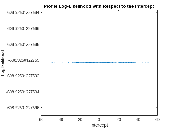
The loglikelihood does not change over the grid of intercept values. The slight
oscillation is a result of the numerical routine used by
infer.