forecast
Forecast sample paths from Markov-switching dynamic regression model
Syntax
Description
YF = forecast(Mdl,Y,numPeriods)YF of a fully specified Markov-switching dynamic regression model Mdl over a forecast horizon of length numPeriods. The forecasted responses represent the continuation of the response data Y.
YF = forecast(Mdl,Y,numPeriods,Name,Value)'X',X specifies exogenous data in the forecast horizon to evaluate regression components in the model.
Examples
Forecast a response path from a two-state Markov-switching dynamic regression model for a 1-D response process. This example uses arbitrary parameter values for the data-generating process (DGP).
Create Fully Specified Model for DGP
Create a two-state discrete-time Markov chain model that describes the regime switching mechanism. Label the regimes.
P = [0.9 0.1; 0.3 0.7];
mc = dtmc(P,'StateNames',["Expansion" "Recession"]);
mc is a fully specified dtmc object.
For each regime, use arima to create an AR model that describes the response process within the regime. Store the submodels in a vector.
mdl1 = arima('Constant',5,'AR',[0.3 0.2],...
    'Variance',2);
mdl2 = arima('Constant',-5,'AR',0.1,...
    'Variance',1);
mdl = [mdl1; mdl2];
mdl1 and mdl2 are fully specified arima objects.
Create a Markov-switching dynamic regression model from the switching mechanism mc and the vector of submodels mdl.
Mdl = msVAR(mc,mdl);
Mdl is a fully specified msVAR object.
Simulate Response Data from DGP
forecast requires enough data before the forecast horizon to initialize the model. Simulate 120 observations from the DGP.
rng(1); % For reproducibility
y = simulate(Mdl,120);
y is a 120-by-1 random path of responses.
Compute Optimal Point Forecasts
Treat the first 100 observations of the simulated response data as the presample for the forecast, and treat the last 20 observations as a holdout sample.
idx0 = 1:100;
idx1 = 101:120;
y0 = y(idx0);
y1 = y(idx1);
Compute 1- through 20-step-ahead optimal point forecasts from the model.
yf = forecast(Mdl,y0,20);
yf is a 20-by-1 vector of optimal point forecasts.
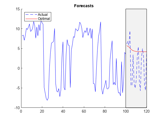
Plot the simulated response data and forecasts.
figure
hold on
plot(idx0,y0,'b');
h = plot(idx1,y1,'b--');
h1 = plot(idx1,yf,'r');
yfill = [ylim fliplr(ylim)];
xfill = [idx0(end) idx0(end) idx1(end) idx1(end)];
fill(xfill,yfill,'k','FaceAlpha',0.05)
legend([h h1],["Actual" "Optimal"],'Location','NorthWest')
title('Forecasts')
hold off
Consider the model in Compute Optimal Point Forecasts.
Create Fully Specified Model for DGP
Create the fully specified Markov-switching dynamic regression model.
P = [0.9 0.1; 0.3 0.7];
mc = dtmc(P,'StateNames',["Expansion" "Recession"]);
mdl1 = arima('Constant',5,'AR',[0.3 0.2],...
    'Variance',2);
mdl2 = arima('Constant',-5,'AR',0.1,...
    'Variance',1);
mdl = [mdl1; mdl2];
Mdl = msVAR(mc,mdl);
Simulate Response Data from DGP
forecast requires enough data before the forecast horizon to initialize the model. Simulate 120 observations from the DGP.
rng(10); % For reproducibility
y = simulate(Mdl,120);
y is a 120-by-1 random path of responses.
Compute Monte Carlo Point Forecasts
Treat the first 100 observations of the simulated response data as the presample for the forecast, and treat the last 20 observations as a holdout sample.
idx0 = 1:100;
idx1 = 101:120;
y0 = y(idx0);
y1 = y(idx1);
Compute 1- through 20-step-ahead optimal point forecasts from the model.
yf1 = forecast(Mdl,y0,20);
yf2 is a 20-by-1 vector of optimal point forecasts.
Compute 1- through 20-step-ahead Monte Carlo point forecasts by returning the estimated forecast error variances.
[yf2,estVar] = forecast(Mdl,y0,20);
yf2 is a 20-by-1 vector of Monte Carlo point forecasts. estVAR is a 20-by-1 vector of corresponding estimated forecast error variances.
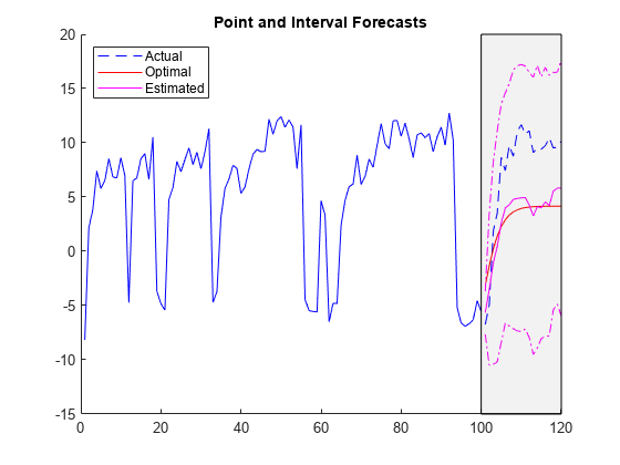
Plot the simulated response data, forecasts, and 95% forecast intervals using the Monte Carlo estimates.
figure
hold on
plot(idx0,y0,'b');
h = plot(idx1,y1,'b--');
h1 = plot(idx1,yf1,'r');
h2 = plot(idx1,yf2,'m');
ciu = yf2 + 1.96*sqrt(estVar); % Upper 95% confidence level
cil = yf2 - 1.96*sqrt(estVar); % Lower 95% confidence level
plot(idx1,ciu,'m-.');
plot(idx1,cil,'m-.');
yfill = [ylim,fliplr(ylim)];
xfill = [idx0(end) idx0(end) idx1(end) idx1(end)];
fill(xfill,yfill,'k','FaceAlpha',0.05)
legend([h h1 h2],["Actual" "Optimal" "Estimated"],...
    'Location',"NorthWest")
title("Point and Interval Forecasts")
hold off
forecast estimates forecasts and corresponding forecast error variances by performing Monte Carlo simulation. You can adjust the number of paths to sample by specifying the 'NumPaths' name-value pair argument. Consider the model in Compute Optimal Point Forecasts.
Create the fully specified Markov-switching dynamic regression model.
P = [0.9 0.1; 0.3 0.7];
mc = dtmc(P,'StateNames',["Expansion" "Recession"]);
mdl1 = arima('Constant',5,'AR',[0.3 0.2],...
    'Variance',2);
mdl2 = arima('Constant',-5,'AR',0.1,...
    'Variance',1);
mdl = [mdl1; mdl2];
Mdl = msVAR(mc,mdl);
Simulate 100 observations from the DGP.
rng(10); % For reproducibility
y = simulate(Mdl,100);
Compute 1- through 20-step-ahead Monte Carlo point forecasts by returning the estimated forecast error variances. Specify 1000 sample paths for the Monte Carlo simulation. Treat the observations y as the presample for the forecast.
[yf,estVar] = forecast(Mdl,y,20,'NumPaths',1000);yf is a 20-by-1 vector of Monte Carlo point forecasts. estVAR is a 20-by-1 vector of corresponding estimated forecast error variances.
Consider a two-state Markov-switching dynamic regression model of the postwar US real GDP growth rate. The model has the parameter estimates presented in [1].
Create Markov-Switching Dynamic Regression Model
Create a fully specified discrete-time Markov chain model that describes the regime switching mechanism. Label the regimes.
P = [0.92 0.08; 0.26 0.74];
mc = dtmc(P,'StateNames',["Expansion" "Recession"]);
Create separate, fully specified AR(0) models for the two regimes.
sigma = 3.34; % Homoscedastic models across states
mdl1 = arima('Constant',4.62,'Variance',sigma^2);
mdl2 = arima('Constant',-0.48,'Variance',sigma^2);
mdl = [mdl1 mdl2];
Create the Markov-switching dynamic regression model from the switching mechanism mc and the state-specific submodels mdl.
Mdl = msVAR(mc,mdl);
Mdl is a fully specified msVAR object.
Load and Preprocess Data
forecast requires observations to initialize the model. Load the US GDP data set.
load Data_GDPData contains quarterly measurements of the US real GDP in the period 1947:Q1–2005:Q2. The period of interest in [1] is 1947:Q2–2004:Q2. For more details on the data set, enter Description at the command line.
Transform the data to an annualized rate series by:
Converting the data to a quarterly rate within the estimation period
Annualizing the quarterly rates
qrate = diff(Data(2:230))./Data(2:229); % Quarterly rate
arate = 100*((1 + qrate).^4 - 1);       % Annualized rate
The transformation drops the first observation.
Forecast US GDP Rates
Forecast the model over a 12-quarter forecast horizon. Initialize the model by supplying the annualized rate series.
numPeriods = 12;
yf = forecast(Mdl,arate,numPeriods);
yf is a 12-by-1 vector of model forecasts. yf(j) is the j-step-ahead optimal point forecast.
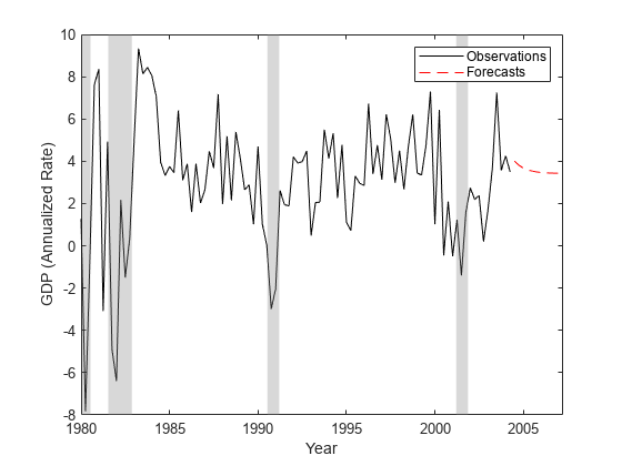
Plot the observed annualized GDP rate from 1980 with the model forecasts.
dates = datetime(dates(3:230),'ConvertFrom','datenum',...
    'Format','yyyy:QQQ','Locale','en_US');
dt1980Q1 = datetime("1980:Q1",'InputFormat','yyyy:QQQ',...
    'Locale','en_US'); % Specify US date format for 1980:Q1.
idx = dates >= dt1980Q1;
figure;
plot(dates(idx),arate(idx),'k',...
    dates(end) + calquarters(1:numPeriods),yf,'r--')
xlabel("Year")
ylabel("GDP (Annualized Rate)")
recessionplot
legend("Observations","Forecasts")
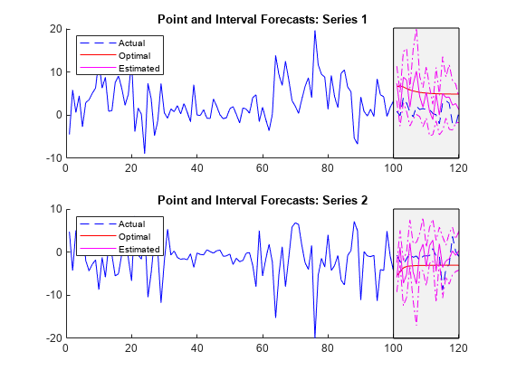
Compute optimal and estimated forecasts and corresponding forecast error covariance matrices from a three-state Markov-switching dynamic regression model for a 2-D VARX response process. This example uses arbitrary parameter values for the DGP.
Create Fully Specified Model for DGP
Create a three-state discrete-time Markov chain model for the switching mechanism.
P = [10 1 1; 1 10 1; 1 1 10];
mc = dtmc(P);
mc is a fully specified dtmc object. dtmc normalizes the rows of P so that they sum to 1.
For each regime, use varm to create a VAR model that describes the response process within the regime. Specify all parameter values.
% Constants
C1 = [1;-1];
C2 = [2;-2];
C3 = [3;-3];

% Autoregression coefficients
AR1 = {};
AR2 = {[0.5 0.1; 0.5 0.5]};
AR3 = {[0.25 0; 0 0] [0 0; 0.25 0]};

% Regression coefficients
Beta1 = [1;-1];
Beta2 = [2 2;-2 -2];
Beta3 = [3 3 3;-3 -3 -3];

% Innovations covariances
Sigma1 = [1 -0.1; -0.1 1];
Sigma2 = [2 -0.2; -0.2 2];
Sigma3 = [3 -0.3; -0.3 3];

% VARX submodels
mdl1 = varm('Constant',C1,'AR',AR1,'Beta',Beta1,'Covariance',Sigma1);
mdl2 = varm('Constant',C2,'AR',AR2,'Beta',Beta2,'Covariance',Sigma2);
mdl3 = varm('Constant',C3,'AR',AR3,'Beta',Beta3,'Covariance',Sigma3);
mdl = [mdl1; mdl2; mdl3];
mdl contains three fully specified varm model objects.
For the DGP, create a fully specified Markov-switching dynamic regression model from the switching mechanism mc and the submodels mdl.
Mdl = msVAR(mc,mdl);
Mdl is a fully specified msVAR model.
Forecast Model Ignoring Regression Component
If you do not supply exogenous data, simulate and forecast ignore the regression components in the submodels. forecast requires enough data before the forecast horizon to initialize the model. Simulate 120 observations from the DGP.
rng('default'); % For reproducibility
Y = simulate(Mdl,120);
Y is a 120-by-2 matrix of simulated responses. Rows correspond to time points, and columns correspond to variables in the system.
Treat the first 100 observations of the simulated response data as the presample for the forecast, and treat the last 20 observations as a holdout sample.
idx0 = 1:100;
idx1 = 101:120;
Y0 = Y(idx0,:); % Forecast sample
Y1 = Y(idx1,:); % Holdout sample
Compute 1- through 20-step-ahead optimal and estimated point forecasts from the model. Compute forecast error covariance matrices corresponding to the estimated forecasts.
YF1 = forecast(Mdl,Y0,20);
[YF2,EstCov] = forecast(Mdl,Y0,20);
YF1 and YF2 are 20-by-2 matrices of optimal and estimated forecasts, respectively. EstCov is a 2-by-2-by-20 array of forecast error covariances.
Extract the forecast error variances of each response for each period in the forecast horizon.
estVar1(:) = EstCov(1,1,:);
estVar2(:) = EstCov(2,2,:);
estVar1 and estVar2 are 1-by-20 vectors of forecast error variances.
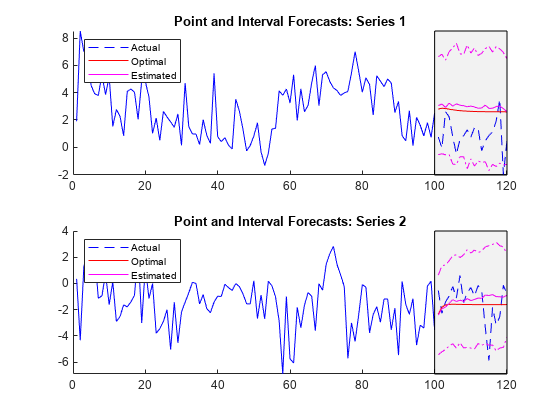
Plot the data, forecasts, and 95% forecast intervals of each variable on separate subplots.
figure

subplot(2,1,1)
hold on
plot(idx0,Y0(:,1),'b');
h = plot(idx1,Y1(:,1),'b--');
h1 = plot(idx1,YF1(:,1),'r');
h2 = plot(idx1,YF2(:,1),'m');
ciu = YF2(:,1) + 1.96*sqrt(estVar1');   % Upper 95% confidence level
cil = YF2(:,1) - 1.96*sqrt(estVar1');   % Lower 95% confidence level
plot(idx1,ciu,'m-.');
plot(idx1,cil,'m-.');
yfill = [ylim,fliplr(ylim)];
xfill = [idx0(end) idx0(end) idx1(end) idx1(end)];
fill(xfill,yfill,'k','FaceAlpha',0.05)
legend([h h1 h2],["Actual" "Optimal" "Estimated"],...
    'Location',"NorthWest")
title("Point and Interval Forecasts: Series 1")
hold off

subplot(2,1,2)
hold on
plot(idx0,Y0(:,2),'b');
h = plot(idx1,Y1(:,2),'b--');
h1 = plot(idx1,YF1(:,2),'r');
h2 = plot(idx1,YF2(:,2),'m');
ciu = YF2(:,2) + 1.96*sqrt(estVar2');   % Upper 95% confidence level
cil = YF2(:,2) - 1.96*sqrt(estVar2');   % Lower 95% confidence level
plot(idx1,ciu,'m-.');
plot(idx1,cil,'m-.');
yfill = [ylim,fliplr(ylim)];
xfill = [idx0(end) idx0(end) idx1(end) idx1(end)];
fill(xfill,yfill,'k','FaceAlpha',0.05)
legend([h h1 h2],["Actual" "Optimal" "Estimated"],...
    'Location',"NorthWest")
title("Point and Interval Forecasts: Series 2")
hold off
Forecast Model Including Regression Component
Simulate exogenous data for the three regressors by generating 120 random observations from the 3-D standard Gaussian distribution.
X = randn(120,3);
Simulate 120 observations from the DGP. Specify the exogenous data for the regression component.
rng('default')
Y = simulate(Mdl,120,'X',X);
Treat the first 100 observations of the simulated response and exogenous data as the presample for the forecast, and treat the last 20 observations as a holdout sample.
idx0 = 1:100;
idx1 = 101:120;
Y0 = Y(idx0,:);
Y1 = Y(idx1,:);
X1 = X(idx1,:);
Compute 1- through 20-step-ahead optimal and estimated point forecasts from the model. Compute forecast error covariance matrices corresponding to the estimated forecasts. Specify the forecast-period exogenous data for the regression component.
YF1 = forecast(Mdl,Y0,20,'X',X1);
[YF2,EstCov] = forecast(Mdl,Y0,20,'X',X1);
estVar1(:) = EstCov(1,1,:);
estVar2(:) = EstCov(2,2,:);
Plot the data, forecasts, and 95% forecast intervals of each variable on separate subplots.
figure

subplot(2,1,1)
hold on
plot(idx0,Y0(:,1),'b');
h = plot(idx1,Y1(:,1),'b--');
h1 = plot(idx1,YF1(:,1),'r');
h2 = plot(idx1,YF2(:,1),'m');
ciu = YF2(:,1) + 1.96*sqrt(estVar1');   % Upper 95% confidence level
cil = YF2(:,1) - 1.96*sqrt(estVar1');   % Lower 95% confidence level
plot(idx1,ciu,'m-.');
plot(idx1,cil,'m-.');
yfill = [ylim,fliplr(ylim)];
xfill = [idx0(end) idx0(end) idx1(end) idx1(end)];
fill(xfill,yfill,'k','FaceAlpha',0.05)
legend([h h1 h2],["Actual" "Optimal" "Estimated"],...
    'Location',"NorthWest")
title("Point and Interval Forecasts: Series 1")
hold off

subplot(2,1,2)
hold on
plot(idx0,Y0(:,2),'b');
h = plot(idx1,Y1(:,2),'b--');
h1 = plot(idx1,YF1(:,2),'r');
h2 = plot(idx1,YF2(:,2),'m');
ciu = YF2(:,2) + 1.96*sqrt(estVar2');   % Upper 95% confidence level
cil = YF2(:,2) - 1.96*sqrt(estVar2');   % Lower 95% confidence level
plot(idx1,ciu,'m-.');
plot(idx1,cil,'m-.');
yfill = [ylim,fliplr(ylim)];
xfill = [idx0(end) idx0(end) idx1(end) idx1(end)];
fill(xfill,yfill,'k','FaceAlpha',0.05)
legend([h h1 h2],["Actual" "Optimal" "Estimated"],...
    'Location',"NorthWest")
title("Point and Interval Forecasts: Series 2")
hold off
Input Arguments
Name-Value Arguments
Output Arguments
Algorithms
Hamilton [2] provides a statistically optimal, one-step-ahead point forecast YF for a Markov-switching dynamic regression model. forecast computes YF iteratively to the forecast horizon when called with a single output. Nonlinearity of the Markov-switching dynamic regression model leads to nonnormal forecast errors, which complicate interval and density forecasts [3]. As a result, forecast switches to Monte Carlo methods when it returns EstCov.
References
[1] Chauvet, M., and J. D. Hamilton. "Dating Business Cycle Turning Points." In Nonlinear Analysis of Business Cycles (Contributions to Economic Analysis, Volume 276). (C. Milas, P. Rothman, and D. van Dijk, eds.). Amsterdam: Emerald Group Publishing Limited, 2006.
[2] Hamilton, J. D. "Analysis of Time Series Subject to Changes in Regime." Journal of Econometrics. Vol. 45, 1990, pp. 39–70.
[3] Krolzig, H.-M. Markov-Switching Vector Autoregressions. Berlin: Springer, 1997.
Version History
Introduced in R2019b