hac
Heteroscedasticity and autocorrelation consistent covariance estimators
Syntax
Description
[
returns a robust covariance matrix estimate, and vectors of corrected standard errors and
OLS coefficient estimates from applying ordinary least squares (OLS) on the multiple linear
regression models EstCoeffCov,se,coeff] = hac(X,y)y = Xβ +
ε under general forms of heteroscedasticity and autocorrelation in the
innovations process ε. y is a vector of response
data and X is a matrix of predictor data.
[
returns a robust covariance matrix estimate, and vectors of corrected standard errors and
OLS coefficient estimates from a fitted multiple linear regression model, as returned by
EstCoeffCov,se,coeff] = hac(Mdl)fitlm.
[
returns a table containing the robust covariance matrix estimate, and a table containing the
corrected standard errors and OLS coefficient estimates, from a fitted multiple linear
regression model of the variables in the input table or timetable.CovTbl,CoeffTbl] = hac(Tbl)
The response variable in the regression is the last table variable, and all other
variables are the predictor variables. To select a different response variable for the
regression, use the ResponseVariable name-value argument. To select
different predictor variables, use the PredictorNames name-value
argument.
[___] = hac(___,
specifies options using one or more name-value arguments in
addition to any of the input argument combinations in previous syntaxes.
Name=Value)hac returns the output argument combination for the
corresponding input arguments.
For example, hac(Tbl,ResponseVariable="GDP",Type="HC") provides
a heteroscedasticity-consistent coefficient covariance estimate of a regression where the
table variable GDP is the response while all other variables are
predictors.
Examples
By default, hac returns the Newey-West coefficient covariance estimate, which is appropriate when residuals from a linear regression fit show evidence of heteroscedasticity and autocorrelation.
Simulate data from a linear model in which the innovations process is heteroscedastic and autocorrelated. Compare coefficient covariance estimates from regular OLS and the Newey-West estimator by using the default options of hac.
Simulate Data
Simulate a 1000-path series of data from the following innovations process.
where and .
rng(1); % For reproducibility
T = 1000;
sigma2 = 0.001*(1:T)';
ut = randn(T,1).*sqrt(sigma2);
eMdl = arima(AR=0.5,Constant=0,Variance=1);
et = filter(eMdl,ut,Y0=0.1);
Simulate responses from the following linear model.
where
X = [1 2] + randn(T,2).*sqrt([1/2 1]);
beta = (1:3)';
y = [ones(T,1) X]*beta + et;
Fit Linear Model
Fit a CLM to the simulated data. Plot the residuals in case order and plot each residual with respect to the previous residual.
Mdl = fitlm(X,y);

tiledlayout(2,1)
nexttile
plotResiduals(Mdl,"caseorder")
nexttile
plotResiduals(Mdl,"lagged")
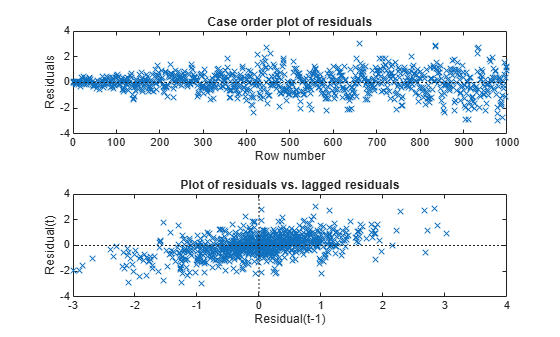
The residuals exhibit heteroscedasticity and autocorrelation.
Compute Newey-West Coefficient Covariance Estimate
Estimate the Newey-West covariance, which accounts for the heteroscedasticity and autocorrelation of the residuals, by passing the data to hac. Return standard errors and coefficients. Compare results against the CLM approach.
[EstCoeffCov,se,coeff] = hac(X,y)
Estimator type: HAC
Estimation method: BT
Bandwidth: 11.1758
Whitening order: 0
Effective sample size: 1000
Small sample correction: on

Coefficient Covariances:

       |  Const      x1       x2
-----------------------------------
 Const |  0.0042  -0.0009  -0.0011
 x1    | -0.0009   0.0012  -0.0000
 x2    | -0.0011  -0.0000   0.0006
EstCoeffCov = 3×3

    0.0042   -0.0009   -0.0011
   -0.0009    0.0012   -0.0000
   -0.0011   -0.0000    0.0006
se = 3×1

    0.0645
    0.0341
    0.0254
coeff = 3×1

    1.0444
    2.0153
    2.9567
EstCoeffCovOLS = Mdl.CoefficientCovariance
EstCoeffCovOLS = 3×3

    0.0045   -0.0012   -0.0013
   -0.0012    0.0012   -0.0000
   -0.0013   -0.0000    0.0007
seOLS = Mdl.Coefficients.SE
seOLS = 3×1

    0.0669
    0.0348
    0.0257
coeffOLS = Mdl.Coefficients.Estimate
coeffOLS = 3×1

    1.0444
    2.0153
    2.9567
Between the CLM and Newey-West approaches, the coefficient estimates are equal, but the standard errors and covariances are different.
Model an automobile's price with its curb weight, engine size, and cylinder bore diameter using the linear model:
Estimate model coefficients and White's robust covariance.
Load the 1985 automobile imports data set import-85.mat, which contains all variables in the matrix X. Collect the variables in the regression model in a table.
load imports-85
varnames = ["CurbWeight" "EngineSize" "Bore" "Price"];

Tbl = array2table(X(:,[7:9 15]),VariableNames=varnames);
Fit the linear model to the data and plot the residuals versus the fitted values.
Mdl = fitlm(Tbl);
plotResiduals(Mdl,"fitted")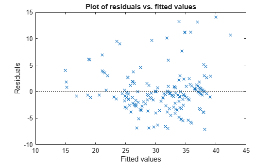
The residuals appear to flare out, which indicates heteroscedasticity.
Use hac to compute the usual OLS coefficient covariance estimate and White's robust covariance estimate.
[LSCov,lsSE,lsCoeff] = hac(Mdl,Type="HC",Weights="CLM", ...
    Display="off") % OLS estimates
LSCov = 4×4

   13.7124    0.0000    0.0120   -4.5609
    0.0000    0.0000   -0.0000   -0.0005
    0.0120   -0.0000    0.0002   -0.0017
   -4.5609   -0.0005   -0.0017    1.8195
lsSE = 4×1

    3.7030
    0.0011
    0.0133
    1.3489
lsCoeff = 4×1

   64.0948
   -0.0087
   -0.0158
   -2.6998
[WhiteCov,whiteSE,whiteCoeff] = hac(Mdl,Type="HC",Weights="HC0", ...
    Display="off") % White's estimates
WhiteCov = 4×4

   15.5122   -0.0008    0.0137   -4.4461
   -0.0008    0.0000   -0.0000   -0.0003
    0.0137   -0.0000    0.0001   -0.0010
   -4.4461   -0.0003   -0.0010    1.5707
whiteSE = 4×1

    3.9385
    0.0011
    0.0105
    1.2533
whiteCoeff = 4×1

   64.0948
   -0.0087
   -0.0158
   -2.6998
The OLS coefficient covariance estimate is not equal to White's robust estimate because the latter accounts for the heteroscedasticity in the residuals.
Model the nominal GNP (GNPN) with consumer price index (CPI), real wages (WR), and the money stock (MS) using the linear model:
Estimate the model coefficients and the Newey-West OLS coefficient covariance matrix.
Load the Nelson Plosser data set Data_NelsonPlosser.mat, which contains the table DataTable. Remove all observations containing at least one NaN and compute the log of the series.
load Data_NelsonPlosser
Tbl = rmmissing(DataTable);
LogTbl = varfun(@log,Tbl);
T = height(LogTbl);
Fit the linear model using the log of all series. Plot the residuals by case order and plot a correlogram of them.
Mdl = fitlm(LogTbl,"log_GNPN ~ 1 + log_CPI + log_WR + log_MS");
resid = Mdl.Residuals.Raw;

figure
tiledlayout(2,1)
nexttile
plotResiduals(Mdl,"caseorder")
axis tight
nexttile
autocorr(resid)
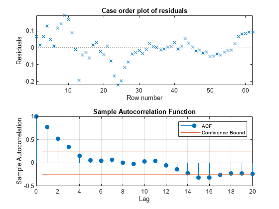
The residual plot exhibits signs of heteroscedasticity, autocorrelation, and possibly model misspecification. The sample autocorrelation function clearly exhibits autocorrelation.
Calculate the lag selection parameter for the standard Newey-West HAC estimate [2].
maxLag = floor(4*(T/100)^(2/9));
Estimate the standard Newey-West OLS coefficient covariance by using hac. Set the bandwidth to maxLag + 1. Display the OLS coefficient estimates, and their standard errors and covariance matrix.
prednames = ["log_CPI" "log_WR" "log_MS"];
[CovTbl,CoeffTbl] = hac(LogTbl,ResponseVariable="log_GNPN", ...
    PredictorVariables=prednames,Bandwidth=maxLag + 1, ...
    Display="full")
Estimator type: HAC
Estimation method: BT
Bandwidth: 4.0000
Whitening order: 0
Effective sample size: 62
Small sample correction: on

Coefficient Estimates:

         |  Coeff     SE
---------------------------
 Const   | -4.3473  0.4297
 log_CPI |  0.9947  0.1001
 log_WR  |  1.3954  0.1283
 log_MS  |  0.0789  0.0625

Coefficient Covariances:

         |  Const   log_CPI   log_WR   log_MS
----------------------------------------------
 Const   |  0.1847  -0.0318  -0.0433   0.0239
 log_CPI | -0.0318   0.0100   0.0027  -0.0043
 log_WR  | -0.0433   0.0027   0.0165  -0.0064
 log_MS  |  0.0239  -0.0043  -0.0064   0.0039
CovTbl=4×4 table
                 Const       log_CPI       log_WR        log_MS
               _________    __________    _________    __________

    Const        0.18468      -0.03177    -0.043323      0.023939
    log_CPI     -0.03177      0.010015    0.0026864    -0.0043025
    log_WR     -0.043323     0.0026864     0.016454     -0.006435
    log_MS      0.023939    -0.0043025    -0.006435     0.0039086
CoeffTbl=4×2 table
                Coeff         SE
               ________    ________

    Const       -4.3473     0.42974
    log_CPI     0.99472     0.10008
    log_WR       1.3954     0.12827
    log_MS     0.078933    0.062519
The first table in the output contains the OLS estimates (, respectively) and their standard errors. The second table is the Newey-West coefficient covariance matrix estimate. For example, . hac returns tables of estimates when you supply a table of data.
Plot the kernel density functions available in hac.
Set domain, x, and range w.
x = (0:0.001:3.2)';
w = zeros(size(x));
Compute the truncated kernel density.
cTR = 2;    % Renormalization constant
TR = (abs(x) <= 1);
TRRn = (abs(cTR*x) <= 1);
wTR = w;
wTR(TR) = 1;
wTRRn = w;
wTRRn(TRRn) = 1;
Compute the Bartlett kernel density.
cBT = 2/3;  % Renormalization constant
BT = (abs(x) <= 1);
BTRn = (abs(cBT*x) <= 1);
wBT = w;
wBT(BT) = 1-abs(x(BT));
wBTRn = w;
wBTRn(BTRn) = 1-abs(cBT*x(BTRn));
Compute the Parzen kernel density.
cPZ = 0.539285;     % Renormalization constant
PZ1 = (abs(x) >= 0) & (abs(x) <= 1/2);
PZ2 = (abs(x) >= 1/2) & (abs(x) <= 1);
PZ1Rn = (abs(cPZ*x) >= 0) & (abs(cPZ*x) <= 1/2);
PZ2Rn = (abs(cPZ*x) >= 1/2) & (abs(cPZ*x) <= 1);
wPZ = w;
wPZ(PZ1) = 1-6*x(PZ1).^2+6*abs(x(PZ1)).^3;
wPZ(PZ2) = 2*(1-abs(x(PZ2))).^3;
wPZRn = w;
wPZRn(PZ1Rn) = 1-6*(cPZ*x(PZ1Rn)).^2 ...
    + 6*abs(cPZ*x(PZ1Rn)).^3;
wPZRn(PZ2Rn) = 2*(1-abs(cPZ*x(PZ2Rn))).^3;
Compute the Tukey-Hanning kernel density.
cTH = 3/4;  % Renormalization constant
TH = (abs(x) <= 1);
THRn = (abs(cTH*x) <= 1);
wTH = w;
wTH(TH) = (1+cos(pi*x(TH)))/2;
wTHRn = w;
wTHRn(THRn) = (1+cos(pi*cTH*x(THRn)))/2;
Compute the quadratic spectral kernel density.
argQS = 6*pi*x/5;
w1 = 3./(argQS.^2);
w2 = (sin(argQS)./argQS)-cos(argQS);
wQS = w1.*w2;
wQS(x == 0) = 1;
wQSRn = wQS;    % Renormalization constant = 1
Plot the kernel densities.
figure
plot(x,[wTR wBT wPZ wTH wQS],LineWidth=2)
hold on
plot(x,w,"k",LineWidth=2)
axis([0 3.2 -0.2 1.2])
grid on
title("\bf HAC Kernels")
legend(["Truncated" "Bartlett" "Parzen" "Tukey-Hanning", ...
    "Quadratic spectral"])
xlabel("Covariance Lag")
ylabel("Weight")
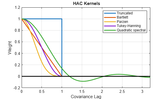
All graphs are truncated at Covariance Lag = 1, except for the quadratic spectral. The quadratic spectral density approaches 0 as Covariance Lag gets large, but does not get truncated.
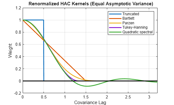
Plot renormalized kernels. Unlike the densities in the previous plot, these have the same asymptotic variance [1].
figure
plot(x,[wTRRn,wBTRn,wPZRn,wTHRn,wQSRn],LineWidth=2)
hold on
plot(x,w,"k",LineWidth=2)
axis([0 3.2 -0.2 1.2])
grid on
title("{\bf Renormalized HAC Kernels} (Equal Asymptotic Variance)")
legend(["Truncated" "Bartlett" "Parzen" "Tukey-Hanning" "Quadratic spectral"])
xlabel("Covariance Lag")
ylabel("Weight")
Examine the effects of changing the bandwidth parameter on the quadratic spectral density.
Assign several bandwidth values to b. Assign the domain to l. Calculate x = l/|b|.
b = (1:5)';
l = (0:0.1:10);
x = bsxfun(@rdivide,repmat(l,[size(b) 1]),b)';
Calculate the quadratic spectral density under the domain for each bandwidth value.
argQS = 6*pi*x/5;
w1 = 3./(argQS.^2);
w2 = (sin(argQS)./argQS)-cos(argQS);
wQS = w1.*w2;
wQS(x == 0) = 1;
Plot the quadratic spectral densities.
figure
plot(l,wQS,LineWidth=2);
grid on
xlabel("Covariance Lag");
ylabel("Quadratic Spectral Density");
title("\bf Change in Bandwidth for Quadratic Spectral Denisty");
legend("Bandwidth = 1","Bandwidth = 2","Bandwidth = 3", ...
    "Bandwidth = 4","Bandwidth = 5");
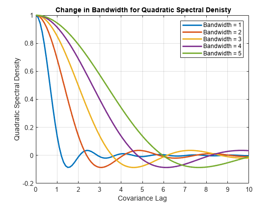
As the bandwidth increases, the kernel imparts more weight to larger lags.
Input Arguments
Name-Value Arguments
Output Arguments
More About
Tips
To reduce bias in HAC estimators, prewhiten the input series [2]. The prewhitening procedure tends to increase estimator variance and mean-squared error, but it can improve confidence interval coverage probabilities and reduce the over-rejection of t statistics.
Algorithms
The original White HC estimator, specified by the settings
Type="HC",Weights="HC0"is justified asymptotically. The other values of theWeightsname-value argument,"HC1","HC2","HC3", and"HC4", are meant to improve small-sample performance. Specify"HC3"or"HC4"in the presence of influential observations (see [6] and [3]).HAC estimators formed using the truncated kernel might not be positive semidefinite in finite samples. [10] proposes using the Bartlett kernel as a remedy, but the resulting estimator is suboptimal in terms of its rate of consistency. The quadratic spectral kernel achieves an optimal rate of consistency.
The default estimation method for HAC bandwidth selection, specified by the
Bandwidthname-value argument, is"AR1MLE", which is generally more accurate, but slower, than the AR(1) alternative"AR1OLS". If you specifyBandwidth="ARMA11",hacfits the model using maximum likelihood.Bandwidth selection models might exhibit sensitivity to the relative scale of the input predictors.
References
[1] Andrews, D. W. K. "Heteroskedasticity and Autocorrelation Consistent Covariance Matrix Estimation." Econometrica. Vol. 59, 1991, pp. 817–858.
[2] Andrews, D. W. K., and J. C. Monohan. "An Improved Heteroskedasticity and Autocorrelation Consistent Covariance Matrix Estimator." Econometrica. Vol. 60, 1992, pp. 953–966.
[3] Cribari-Neto, F. "Asymptotic Inference Under Heteroskedasticity of Unknown Form." Computational Statistics & Data Analysis. Vol. 45, 2004, pp. 215–233.
[4] den Haan, W. J., and A. Levin. "A Practitioner's Guide to Robust Covariance Matrix Estimation." In Handbook of Statistics. Edited by G. S. Maddala and C. R. Rao. Amsterdam: Elsevier, 1997.
[5] Frank, A., and A. Asuncion. UCI Machine Learning Repository. Irvine, CA: University of California, School of Information and Computer Science. https://archive.ics.uci.edu/, 2012.
[6] Gallant, A. R. Nonlinear Statistical Models. Hoboken, NJ: John Wiley & Sons, Inc., 1987.
[7] Kutner, M. H., C. J. Nachtsheim, J. Neter, and W. Li. Applied Linear Statistical Models. 5th ed. New York: McGraw-Hill/Irwin, 2005.
[8] Long, J. S., and L. H. Ervin. "Using Heteroscedasticity-Consistent Standard Errors in the Linear Regression Model." The American Statistician. Vol. 54, 2000, pp. 217–224.
[11] Newey, W. K, and K. D. West. “Automatic Lag Selection in Covariance Matrix Estimation.” The Review of Economic Studies. Vol. 61 No. 4, 1994, pp. 631–653.
[12] White, H. "A Heteroskedasticity-Consistent Covariance Matrix and a Direct Test for Heteroskedasticity." Econometrica. Vol. 48, 1980, pp. 817–838.
[13] White, H. Asymptotic Theory for Econometricians. New York: Academic Press, 1984.