Simulate Radar Ghosts Due to Multipath Return
This example shows how to simulate ghost target detections and tracks due to multipath reflections, where signal energy is reflected off another target before returning to the radar. In this example you will simulate ghosts with both a statistical radar model and a transceiver model that generates IQ signals.
Motivation
Many highway scenarios involve not only other cars, but also barriers and guardrails. Consider the simple highway created using the Driving Scenario Designer app. For more information on how to model barriers see the Sensor Fusion Using Synthetic Radar and Vision Data example. Use the helperSimpleHighwayScenarioDSD function exported from the Driving Scenario Designer to get the highway scenario and a handle to the ego vehicle.
% Set random seed for reproducible results
rndState = rng('default');

% Create scenario using helper
[scenario, egoVehicle] = helperSimpleHighwayScenarioDSD();
To model the detections generated by a forward-looking automotive radar, use the radarDataGenerator System object™. Use a 77 GHz center frequency, which is typical for automotive radar. Generate detections up to 150 meters in range and with a radial speed up to 100 m/s.
% Automotive radar system parameters
freq = 77e9; % Hz
rgMax = 150; % m
spMax = 100; % m/s
rcs = 10;    % dBsm

azRes = 4;   % deg
rgRes = 2.5; % m
rrRes = 0.5; % m/s

% Create a forward-looking automotive radar
rdg = radarDataGenerator(1, 'No scanning', ...
    'UpdateRate', 10, ...
    'MountingLocation', [3.4 0 0.2], ...
    'CenterFrequency', freq, ...
    'HasRangeRate', true, ...
    'FieldOfView', [70 5], ...
    'RangeLimits', [0 rgMax], ...
    'RangeRateLimits', [-spMax spMax], ...
    'HasRangeAmbiguities',true, ...
    'MaxUnambiguousRange', rgMax, ...
    'HasRangeRateAmbiguities',true, ...
    'MaxUnambiguousRadialSpeed', spMax, ...
    'ReferenceRange', rgMax, ...
    'ReferenceRCS',rcs, ...
    'AzimuthResolution',azRes, ...
    'RangeResolution',rgRes, ...
    'RangeRateResolution',rrRes, ...
    'TargetReportFormat', 'Detections', ...
    'Profiles',actorProfiles(scenario));

% Create bird's eye plot and detection plotter function
[~,detPlotterFcn] = helperSetupBEP(egoVehicle,rdg);
title('Free Space (no multipath)');

% Generate raw detections
time = scenario.SimulationTime;
tposes = targetPoses(egoVehicle);
[dets,~,config] = rdg(tposes,time);

% Plot detections
detPlotterFcn(dets,config);
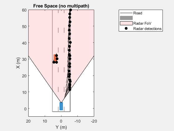
This figure shows the locations of the detections along the target vehicle as well as along the side of the barrier. However, detections are not always so well-behaved. One phenomenon that can pose considerable challenges to radar engineers is multipath. Multipath is when the signal not only propagates directly to the intended target and back to the radar but also includes additional reflections off objects in the environment.
Multipath Reflections
When a radar signal propagates to a target of interest it can arrive through various paths. In addition to the direct path from the radar to the target and then back to the radar, there are other possible propagation paths. The number of paths is unbounded, but with each reflection, the signal energy decreases. Commonly, a propagation model considering three-bounce paths is used to model this phenomenon.
To understand the three-bounce model, first consider the simpler one-bounce and two-bounce paths, as shown in these figures.
One-Bounce Path
The one-bounce path propagates from the radar (1) to the target (2) and then is reflected from the target (2) back to the radar. This is often referred to as the direct or line-of-sight path.
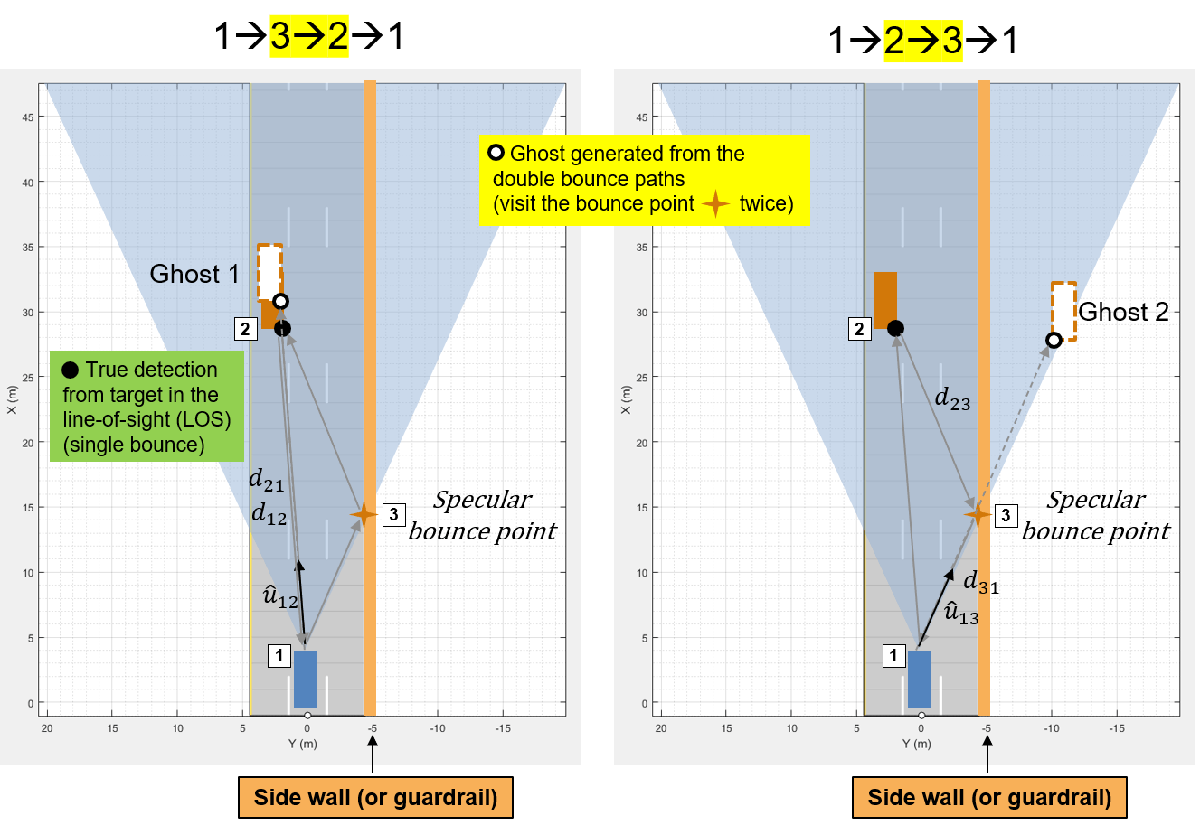
Two-Bounce Paths
In this case, there are two unique propagation paths that consist of two bounces.
The first two-bounce path propagates from the radar (1) to a reflecting surface (3), then to the target (2) before returning to the radar (1). Because the signal received at the radar arrives from the last bounce from the true target, it generates ghost detections along the same direction as the true target. Because the path length for this propagation is longer, it appears at a farther range than the true target detections.
The second two-bounce path propagates from the radar (1) to the target (2), then to the reflecting surface (3) before returning to the radar (1). In this case, the ghost detections appear on the other side of the reflecting surface as the radar receives the reflected signal in that direction.
Notice that the path length for both two-bounce paths is the same. As a result, the measured range and range rate for these paths will be the same as well.
Three-Bounce Path

The three-bounce path reflects off the barrier twice. This path never propagates directly to the target or directly back to the radar. The three-bounce ghost detections appear on the other side of the reflecting surface as the radar receives the reflected signal in that direction. Additionally, it has the longest propagation path of the three-bounce paths and therefore has the longest measured range of the three paths. This path corresponds to a mirror reflection of the true target on the other side of the barrier.
Model Ghost Target Detections
Set the HasGhosts property on the radarDataGenerator to model the detections generated from these three-bounce paths.
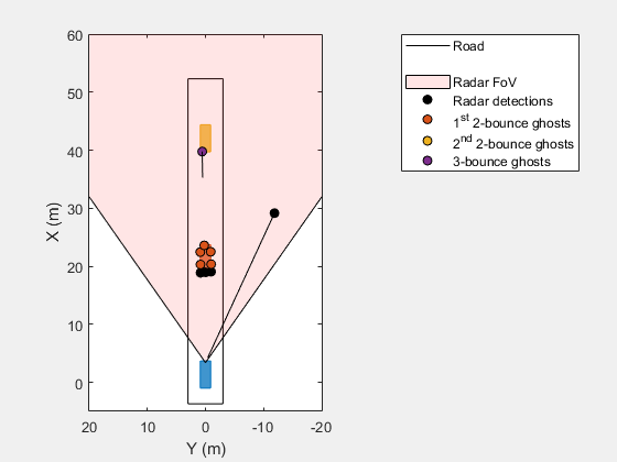
% Enable ghost target model
release(rdg);
rdg.HasGhosts = true;

% Generate raw detections
time = scenario.SimulationTime;
tposes = targetPoses(egoVehicle);
[dets,~,config] = rdg(tposes,time);

% Plot detections
detPlotterFcn(dets,config);
title('Simple Multipath Environment');
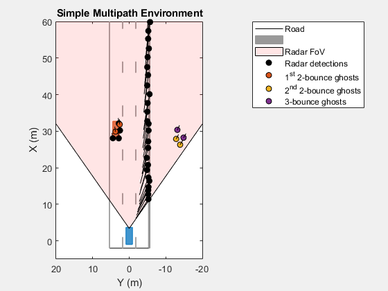
This figure reproduces the analysis of the three propagation paths. The first two-bounce ghosts lie in the direction of the target at a slightly longer range than the direct-path detections. The second two-bounce and three-bounce ghosts lie in the direction of the mirrored image of the target generated by the reflection from the barrier.
Ghost Tracks
Because the range and velocities of the ghost target detections are like the range and velocity of the true targets, they have kinematics that are consistent for a tracker that is configured to track the true target detections. This consistency between the kinematics of real and ghost targets results in tracks being generated for the ghost target on the other side of the barrier.
Set the TargetReportFormat property on radarDataGenerator to Tracks to model the tracks generated by a radar in the presence of multipath.
% Output tracks instead of detections
release(rdg);
rdg.TargetReportFormat = 'Tracks';
rdg.ConfirmationThreshold = [2 3];
rdg.DeletionThreshold = [5 5];
FilterInitializationFcn = 'initcvekf'; % constant-velocity EKF

% Create a new bird's eye plot to plot the tracks
[bep,trkPlotterFcn] = helperSetupBEP(egoVehicle,rdg);
title('Simple Multipath Environment');

% Run simulation
restart(scenario);
scenario.StopTime = 7.5;
while advance(scenario)
    time = scenario.SimulationTime;
    tposes = targetPoses(egoVehicle);

    % Generate tracks
    [trks,~,config] = rdg(tposes,time);

    % Filter out tracks corresponding to static objects (e.g. barrier)
    dyntrks = helperKeepDynamicObjects(trks, egoVehicle);

    % Visualize dynamic tracks
    helperPlotScenario(bep,egoVehicle);
    trkPlotterFcn(dyntrks,config);
end
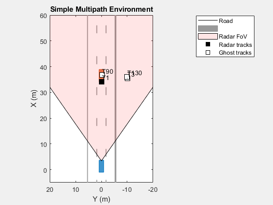
This figure shows the confirmed track positions using square markers. The tracks corresponding to static objects (for example a barrier) are not plotted. Notice that there are multiple tracks associated with the lead car. The tracks that overlay the lead car correspond to the true detection and the first two-bounce ghost. The tracks that lie off of the road on the other side of the guardrail correspond to the second two-bounce and three-bounce ghosts.
The track velocities are indicated by the length and direction of the vectors pointing away from the track position (these are small because they are relative to the ego vehicle). Ghost detections may fool a tracker because they have kinematics like the kinematics of the true targets. These ghost tracks can be problematic as they add an additional processing load to the tracker and can confuse control decisions using the target tracks.
Model IQ Signals
In the previous free-space and multipath simulations in this example, you used measurement-level radar models to generate detections and tracks. Now, use the radarTransceiver System object to generate time-domain IQ signals. Create an equivalent radarTransceiver directly from the radarDataGenerator.
The statistical radar has the following range and range-rate (Doppler) parameters which determine the constraints for the waveform used by the radarTransceiver.
rgMax = rdg.RangeLimits(2) % mrgMax = 150
spMax = rdg.RangeRateLimits(2) % m/sspMax = 100
Compute the pulse repetition frequency (PRF) that will satisfy the range rate for the radar.
lambda = freq2wavelen(rdg.CenterFrequency);
prf = 2*speed2dop(2*spMax,lambda);
Compute the number of pulses needed to satisfy the range-rate resolution requirement.
rrRes = rdg.RangeRateResolution
rrRes =
0.5000
dopRes = 2*speed2dop(rrRes,lambda);
numPulses = 2^nextpow2(prf/dopRes)
numPulses =
512
prf = dopRes*numPulses
prf =
1.3150e+05
Confirm that the unambiguous range that corresponds to this PRF is beyond the maximum range limit.
rgUmb = time2range(1/prf)
rgUmb =
1.1399e+03
Re-set some properties of the radarDataGenerator for better comparison to IQ results from the radarTransceiver.
release(rdg);

% Set the range and range-rate ambiguities according to desired PRF and
% number of pulses
rdg.MaxUnambiguousRange = rgUmb;
rdg.MaxUnambiguousRadialSpeed = spMax;

% Set the statistical radar to report clustered detections to compare to
% the IQ video from the radar transceiver.
rdg.TargetReportFormat = 'Clustered detections';
rdg.DetectionCoordinates = 'Body';
Construct the equivalent radarTransceiver directly from the radarDataGenerator. By default, the radarTransceiver uses a unit-gain rectangular antenna pattern with azimuth and elevation beamwidths equal to the azimuth and elevation resolutions of the radarDataGenerator. To simulate a radar with a transmit pattern that covers the desired field of view, first set the azimuth resolution of the radarDataGenerator equal to the field of view.
azRes = rdg.AzimuthResolution;
rdg.AzimuthResolution = rdg.FieldOfView(1);

% Construct the radar transceiver from the radar data generator
rtxrx = radarTransceiver(rdg)
rtxrx =
radarTransceiver with properties:
Waveform: [1×1 phased.RectangularWaveform]
Transmitter: [1×1 phased.Transmitter]
TransmitAntenna: [1×1 phased.Radiator]
ReceiveAntenna: [1×1 phased.Collector]
Receiver: [1×1 phased.ReceiverPreamp]
MechanicalScanMode: 'None'
ElectronicScanMode: 'None'
MountingLocation: [3.4000 0 0.2000]
MountingAngles: [0 0 0]
NumRepetitionsSource: 'Property'
NumRepetitions: 512
RangeLimitsSource: 'Property'
RangeLimits: [0 150]
RangeOutputPort: false
TimeOutputPort: false
% Restore the desired azimuth resolution for the statistical radar
rdg.AzimuthResolution = azRes;
The statistical radar emulates the use of a uniform linear array (ULA) to form multiple receive beams, as needed to achieve the specified azimuth resolution. The number or elements required is determined by the radar's azimuth resolution and wavelength, and can be found with the beamwidth2ap function.
numRxElmt = ceil(beamwidth2ap(rdg.AzimuthResolution,lambda,0.8859)/(lambda/2))
numRxElmt =
26
Attach a ULA to the receive antenna of the radarTransceiver.
elmt = rtxrx.ReceiveAntenna.Sensor;
rxarray = phased.ULA(numRxElmt,lambda/2,'Element',elmt);
rtxrx.ReceiveAntenna.Sensor = rxarray;
Generate IQ Samples
Use the helper3BounceGhostPaths function to compute the three-bounce paths for the target and sensor positions from the multipath scenario.
restart(scenario);
tposes = targetPoses(egoVehicle);

% Generate 3-bounce propagation paths for the targets in the scenario
paths = helper3BounceGhostPaths(tposes,rdg);
Use the radarTransceiver to generate the baseband sampled IQ data received by the radar.
time = scenario.SimulationTime; % Current simulation time
Xcube = rtxrx(paths,time);      % Generate IQ data for transceiver from the 3-bounce path model
Range and Doppler Processing
The received data cube has the three-dimensions: fast-time samples, receive antenna element, and slow-time samples.
size(Xcube)
ans = 1×3

    64    26   512
Use the phased.RangeDopplerResponse System object to perform range and Doppler processing along the first and third dimensions of the data cube.
rngdopproc = phased.RangeDopplerResponse( ...
    'RangeMethod','Matched filter', ...
    'DopplerOutput','Speed', ...
    'PropagationSpeed',rtxrx.ReceiveAntenna.PropagationSpeed, ...
    'OperatingFrequency',rtxrx.ReceiveAntenna.OperatingFrequency, ...
    'SampleRate',rtxrx.Receiver.SampleRate);
mfcoeff = getMatchedFilter(rtxrx.Waveform);
[Xrngdop,rggrid,rrgrid] = rngdopproc(Xcube,mfcoeff);
Beamforming
Use the phased.PhaseShiftBeamformer System object to form beams from the receive antenna array elements along the second dimension of the data cube.
azFov = rdg.FieldOfView(1);
anggrid = -azFov/2:azFov/2;
bmfwin = @(N)normmax(taylorwin(N,5,-60));
beamformer = phased.PhaseShiftBeamformer( ...
        'Direction',[anggrid;0*anggrid],...
        'SensorArray',rtxrx.ReceiveAntenna.Sensor, ...
        'OperatingFrequency',rtxrx.ReceiveAntenna.OperatingFrequency);
Xbfmrngdop = Xrngdop;
[Nr,Ne,Nd] = size(Xbfmrngdop);
Xbfmrngdop = permute(Xbfmrngdop,[1 3 2]); % Nr x Nd x Ne
Xbfmrngdop = reshape(Xbfmrngdop,[],Ne);
Xbfmrngdop = beamformer(Xbfmrngdop.*bmfwin(Ne)');
Xbfmrngdop = reshape(Xbfmrngdop,Nr,Nd,[]); % Nr x Nd x Nb
Xbfmrngdop = permute(Xbfmrngdop,[1 3 2]); % Nr x Nb x Nd
Use the helperPlotBeamformedRangeDoppler function to plot the range-angle map from the beamformed, range, and Doppler processed data cube.
helperPlotBeamformedRangeDoppler(Xbfmrngdop,rggrid,anggrid,rtxrx);

The local maxima of the received signals correspond to the location of the target vehicle, the guardrail, and the ghost image of the target vehicle on the other side of the guardrail. Show that measurement-level detections generated by radarDataGenerator are consistent with the peaks in the range-angle map generated by the equivalent radarTransceiver.
Use the helperPlayStatAndIQMovie function to compare the measurement-level detections and IQ processed video for the duration of this scenario.
helperPlayStatAndIQMovie(scenario,egoVehicle,rtxrx,rdg,rngdopproc,beamformer,bmfwin);
Multipath Ground Bounce
Multipath ghost detections can be used at times to see objects in the road that would otherwise not be detected by the radar due to occlusion. One example is the detection of an occluded vehicle due to multipath off of the road surface. Use the helperGroundBounceScenarioDSD function to create a scenario where a slower moving vehicle in the same lane as the ego vehicle is occluded by another vehicle directly in front of the radar.
[scenario, egoVehicle] = helperGroundBounceScenarioDSD;
ax3d = helperRadarChasePlot(egoVehicle);
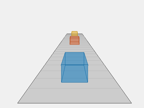
The yellow car is occluded by the red car. A line of sight does not exist between the blue ego car's forward looking-radar and the yellow car.
viewLoc = [scenario.Actors(2).Position(1)-10 -10];
chasePlot(egoVehicle,'ViewLocation',viewLoc,'ViewHeight',0,'ViewYaw',40,'Parent',ax3d);

Multipath can pass through the space between the underside of a car and the surface of the road.
Reuse the radarDataGenerator to generate ghost target detections due to multipath between the vehicles and the road surface. Use the helperRoadProfiles and helperRoadPoses functions to include the road surface in the list of targets modeled in the scenario to enable multipath between the road surface and the vehicles.
release(rdg);
rdg.RangeRateResolution = 0.5;
rdg.FieldOfView(2) = 10;
rdg.TargetReportFormat = 'Detections';

tprofiles = actorProfiles(scenario);
rdprofiles = helperRoadProfiles(scenario);
rdg.Profiles = [tprofiles;rdprofiles];

% Create bird's eye plot and detection plotter function
[bep,detPlotterFcn] = helperSetupBEP(egoVehicle,rdg);
[ax3d,detChasePlotterFcn] = helperRadarChasePlot(egoVehicle,rdg);
camup(ax3d,[0 0 1]);
pos = egoVehicle.Position+[-5 -5 0];
campos(ax3d,pos);
camtarget(ax3d,[15 0 0]);

% Generate clustered detections
time = scenario.SimulationTime;
tposes = targetPoses(egoVehicle);
rdposes = helperRoadPoses(egoVehicle);
poses = [tposes rdposes];

[dets,~,config] = rdg(poses,time);

% Plot detections
dyndets = helperKeepDynamicObjects(dets,egoVehicle);
detPlotterFcn(dyndets,config);
The detection from the occluded car is possible due to the three-bounce path that exists between the road surface and the underside of the red car.
% Find the 3-bounce detection from the occluded car
i3 = find(cellfun(@(d)d.ObjectAttributes{1}.BouncePathIndex,dyndets)==3);
det3 = dyndets{i3};

% Plot the 3-bounce path between the radar and the occluded car
iBncTgt = find([poses.ActorID]==det3.ObjectAttributes{1}.BounceTargetIndex);
iTgt = find([poses.ActorID]==det3.ObjectAttributes{1}.TargetIndex);
pos = [rdg.MountingLocation;poses(iBncTgt).Position;poses(iTgt).Position]+egoVehicle.Position;
hold(ax3d,'on');
plot3(ax3d,pos(:,1),pos(:,2),pos(:,3),'r-*','LineWidth',2);
campos(ax3d,[-6 -15 2]); camtarget(ax3d,[17 0 0]);
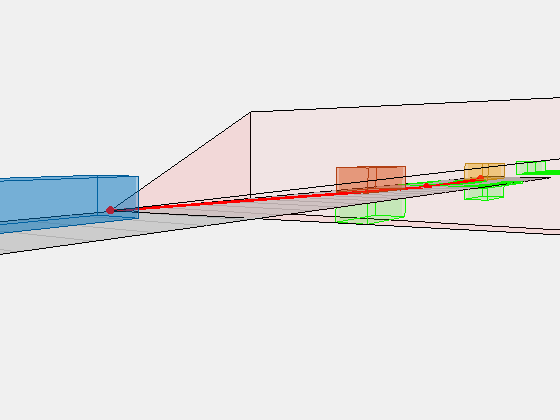
This figure shows the three-bounce path as the red line. Observe that a bounce path between the radar and the occluded yellow car exists by passing below the underside of the red car.
% Show bounce path arriving at the occluded yellow car
campos(ax3d,[55 -10 3]); camtarget(ax3d,[35 0 0]);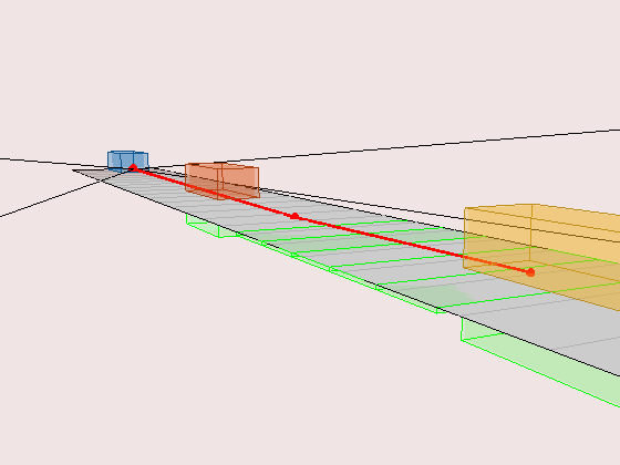
This figure shows the three-bounce path arriving at the occluded yellow car after bouncing off of the road surface.
Summary
In this example, you learned how ghost target detections arise from multiple reflections that can occur between the radar and a target. An automotive radar scenario was used to highlight a common case where ghost targets are generated by a guardrail in the field of view of the radar. As a result, there are four unique bounce paths which can produce these ghost detections. The kinematics of the ghost target detections are like the detections of true targets, and as a result, these ghost targets can create ghost tracks which can add additional processing load to a tracker and may confuse control algorithms using these tracks. The radarTransceiver can be used to generate higher-fidelity IQ data that is appropriate as input to detection and tracking algorithms.
% Restore random state
rng(rndState);
Supporting Functions
helperKeepDynamicObjects
function dynrpts = helperKeepDynamicObjects(rpts,egoVehicle)
% Filter out target reports corresponding to static objects (e.g. guardrail)
%
% This is a helper function and may be removed or modified in a future
% release.

dynrpts = rpts;
if ~isempty(rpts)
    if iscell(rpts)
        vel = cell2mat(cellfun(@(d)d.Measurement(4:end),rpts(:)','UniformOutput',false));
    else
        vel = cell2mat(arrayfun(@(t)t.State(2:2:end),rpts(:)','UniformOutput',false));
    end
    vel = sign(vel(1,:)).*sqrt(sum(abs(vel(1:2,:)).^2,1));
    egoVel = sign(egoVehicle.Velocity(1))*norm(egoVehicle.Velocity(1:2));
    gndvel = vel+egoVel; % detection speed relative to ground
    isStatic = gndvel > -4 & ... greater than 4 m/s departing and,
        gndvel < 8; % less than 8 m/s closing speed
    dynrpts = rpts(~isStatic);
end
end
normmax
function y = normmax(x)
if all(abs(x(:))==0)
    y = ones(size(x),'like',x);
else
    y = x(:)/max(abs(x(:)));
end
end