Automate Real-Time Testing for Highway Lane Following Controller
This example shows how to automate the testing of a lane following controller deployed to a Speedgoat® real-time target machine using Simulink® Test™. In this example, you:
Deploy the highway lane following controller to a Speedgoat machine using Simulink Real-Time™.
Perform automated testing of the deployed application using Simulink Test.
The lane following controller is a fundamental component in highway driving applications, as it combines lateral and longitudinal controls for an ego vehicle. This critical component is most commonly deployed to a real-time processor. This example shows how you can deploy the lane following controller to a Speedgoat real-time machine. It also shows how you can reuse the desktop simulation test cases and automate regression testing for the deployed controller. This example builds on the Generate Code for Highway Lane Following Controller example.
System Configuration
This example uses a hardware setup that primarily consists of two machines, a host and a target, connected by ethernet.
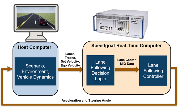
This example uses this hardware configuration:
Target — Speedgoat Performance Real-Time machine with an Intel® Core™ i7 4.2 GHz, running Simulink Real-Time operating system. For more information, see Speedgoat Performance Real-Time Target Machine.
Host — Intel® Xeon® 3.60GHz, running a Windows® 64-bit operating system.
Ethernet cable connecting the target to the host.
The target runs the lane following decision logic and lane following controller. It sends steering angle and acceleration signals to the host using the User Datagram Protocol (UDP) over ethernet.
The host sets up the simulation environment, configures the test scenarios, and models the vehicle dynamics of the ego vehicle. It sends signals carrying information about lanes, tracks, ego velocity, and set velocity to the target using UDP. It receives the steering angle and acceleration to generate the ego pose from the target using UDP.
Using this setup, you can deploy the lane following controller to the target, run the host model for a test scenario, and log and visualize simulation results.
In this example, you:
Review the simulation test bench model — The model contains the scenario, controls, vehicle dynamics, and metrics to assess functionality. The metric assessments integrate the test bench model with Simulink Test for automated testing.
Partition and explore host and target models — The simulation test bench model is partitioned into two models. One runs on the host machine, and the other is used for deployment to the target machine.
Deploy the target model — Configure and deploy the lane following controller model to the target machine using Simulink Real-Time.
Simulate host model and visualize results — Configure the host model with a test scenario. Simulate the model and visualize the results.
Explore the test manager file — Explore the configured test manager file that enables you to automate the testing of the deployed lane following controller.
Automate testing — Run the test suite using the test manager and analyze the test report.
Review Simulation Test Bench Model
This example uses the test bench model from Generate Code for Highway Lane Following Controller, as shown in this figure.
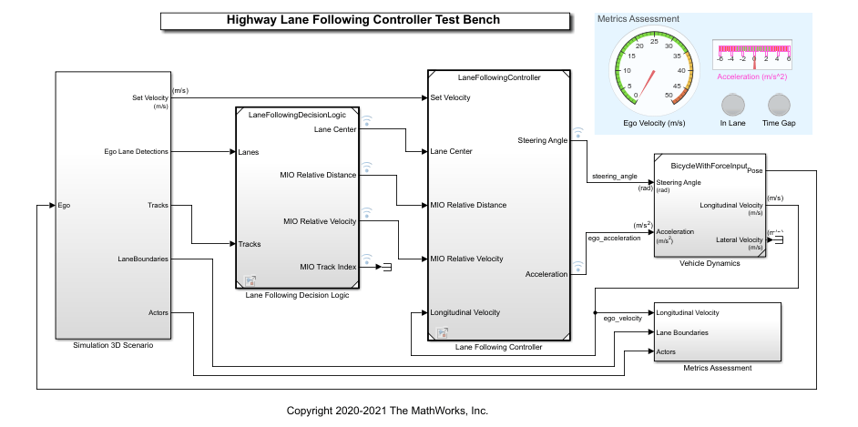
This simulation test bench model contains these subsystems:
Simulation 3D Scenario— Specifies the road, vehicles, and vision detection generator used for simulation.Lane Following Decision Logic— Specifies the lateral and longitudinal decision logic, and provides lane center information and most important object (MIO) related information to the controller.Lane Following Controller— Specifies the path-following controller that generates control commands to steer the ego vehicle.Vehicle Dynamics— Specifies the dynamic model for the ego vehicle.Metrics Assessment— Assesses system-level behavior.
Partition and Explore Host and Target Models
The test bench model is partitioned into host and target models. Explore these models.
Explore Host Model
The host model contains the Simulation 3D Scenario, Vehicle Dynamics, and Metrics Assessment subsystems of the highway lane following application. The model also configures the UDP interface using the UDP Data Send and UDP Data Receive subsystems. Open the host model.
open_system("RTHLFControllerHost")
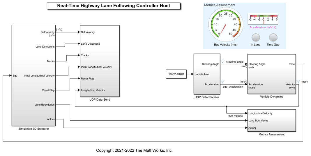
The Simulation 3D Scenario subsystem configures the road network, sets vehicle positions, and packs truth data into detections. For more information see Generate Code for Highway Lane Following Controller. Open the Simulation 3D Scenario subsystem.
open_system("RTHLFControllerHost/Simulation 3D Scenario")

This subsystem also sets the initial velocity of the ego vehicle, and generates the reset flag using a MATLAB® Function block. Use this flag to reset the internal states of the deployed application before you run the simulation.
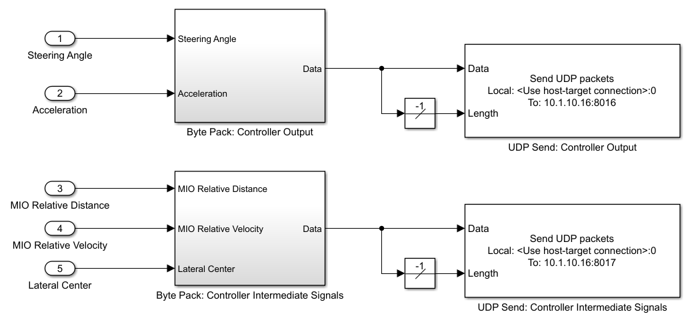
The UDP Data Send subsystem contains Byte Packing (Simulink Real-Time) and UDP Send (Simulink Real-Time) blocks from the Simulink Real-Time library. Open the UDP Data Send subsystem.
open_system("RTHLFControllerHost/UDP Data Send")
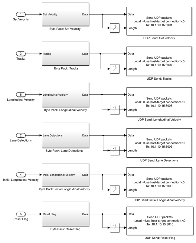
Each Byte Pack subsystem contains a Byte Packing block that converts one or more signals of user-selectable data types to a single vector of varying data types. Each UDP Send block sends the data from the corresponding Byte Pack subsystem over a UDP network to the specified IP address and port. You must configure these UDP Send blocks with the IP address and port number of the target machine.
This list defines the specifications of the data signals.
Set Velocity— 8-byte doubleLongitudinal Velocity— 8-byte doubleInitial Longitudinal Velocity— 8-byte doubleReset Flag— 8-byte doubleTracks— 268-byte Simulink bus structureLane Detections— 32-byte Simulink bus structure
This example sets the maximum number of tracks to 5. You can update this value when you use a different test scenario.
The UDP Data Receive subsystem contains UDP Receive (Simulink Real-Time) and Byte Unpacking (Simulink Real-Time) blocks from the Simulink Real-Time library. Open the UDP Data Receive subsystem.
open_system("RTHLFControllerHost/UDP Data Receive")
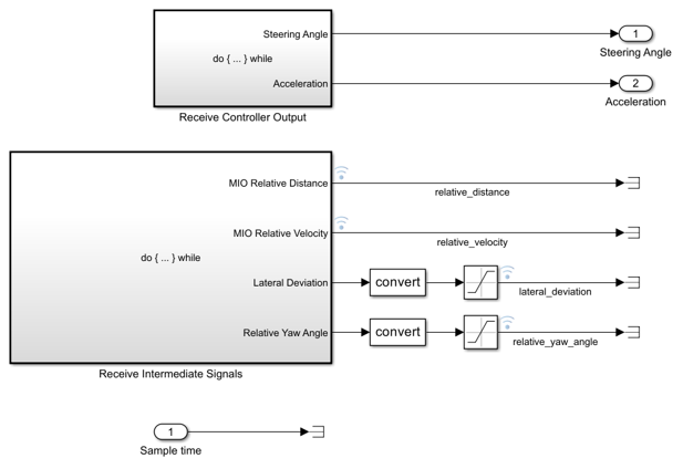
This subsystem contains two additional subsystems:
Receive Controller Output— Receives and unpacks the controller outputs sent from the target machine.
Receive Intermediate Signals— Receives and unpacks the intermediate signals from the target machine.
The Vehicle Dynamics subsystem contains a dynamic model for the ego vehicle.
open_system("RTHLFControllerHost/Vehicle Dynamics")
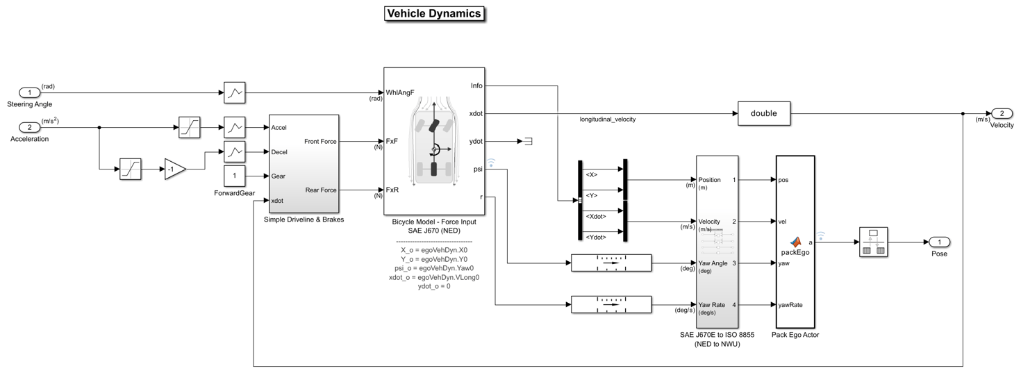
The Vehicle Dynamics subsystem implements a Bicycle Model for the ego vehicle. The subsystem takes controller outputs and estimates the ego vehicle pose.
The Metrics Assessment subsystem is based on the subsystem used in the Generate Code for Highway Lane Following Controller example.
To perform the real-time simulation, the host model runs with simulation pacing set to 1. For more information, see Simulation Pacing Options (Simulink).
Explore Target Model
The target model contains the Highway Lane Following Controller subsystem, along with UDP interfaces. Open the target model.
open_system("RTHLFControllerTarget")
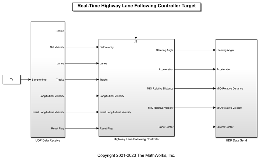
The target model contains these subsystems:
UDP Data Receive— Receives data required for highway lane following controller model to run.Highway Lane Following Controller— Enabled subsystem that contains the lane following decision logic and lane following controller algorithms.UDP Data Send— Sends the outputs of the controller to the host model, which are required byVehicle Dynamicssubsystem of the host model.
The UDP Data Receive subsystem contains UDP Receive and Byte Unpacking blocks from Simulink Real-Time library. Open the UDP Data Receive subsystem.
open_system("RTHLFControllerTarget/UDP Data Receive")
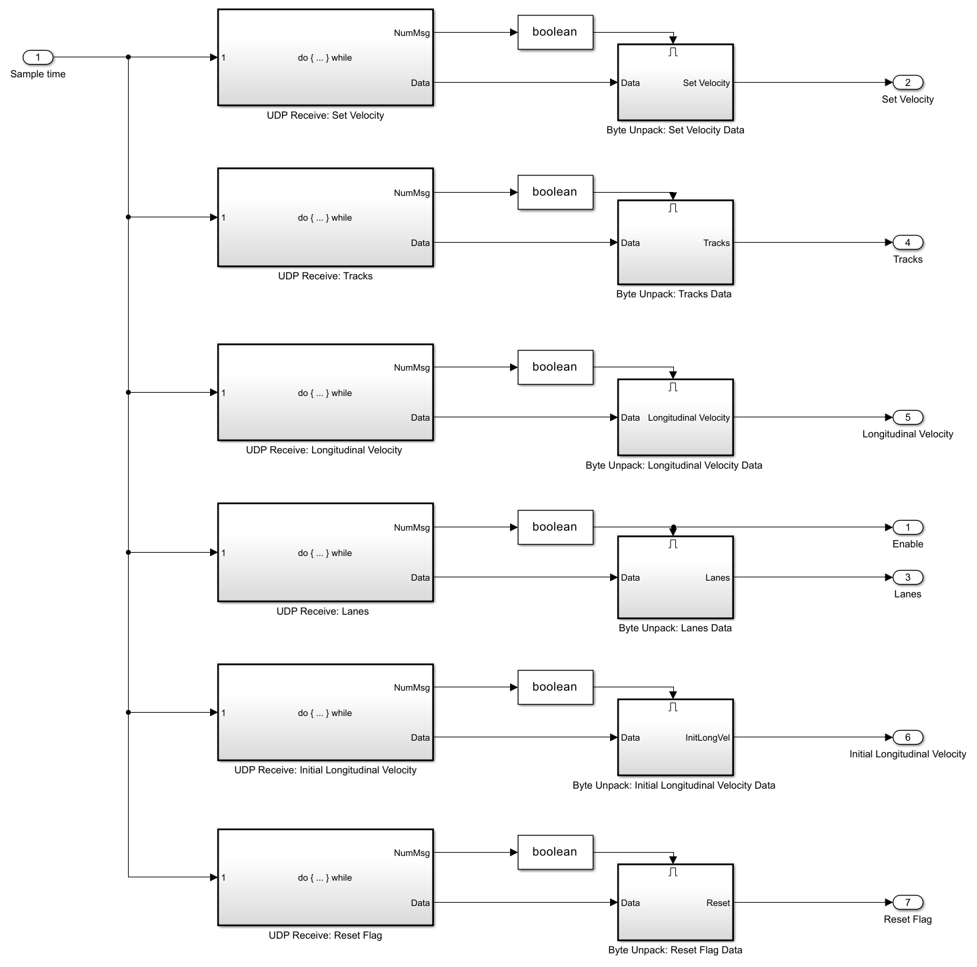
This subsystem receives data frames from the host machine, and deconstructs them using the Byte Unpack subsystems.
The UDP Data Send subsystem contains Byte Packing and UDP Send blocks from Simulink Real-Time library. Open the UDP Data Send subsystem.
open_system("RTHLFControllerTarget/UDP Data Send")
This subsystem sends the controller outputs, Steering Angle and Acceleration, to the host machine using a UDP Send block. It also sends some internal signals used for plotting.
The Highway Lane Following Controller subsystem is an enabled subsystem that enables execution of the controller algorithm upon receiving data from the host machine. Open the Highway Lane Following Controller subsystem.
open_system("RTHLFControllerTarget/Highway Lane Following Controller")
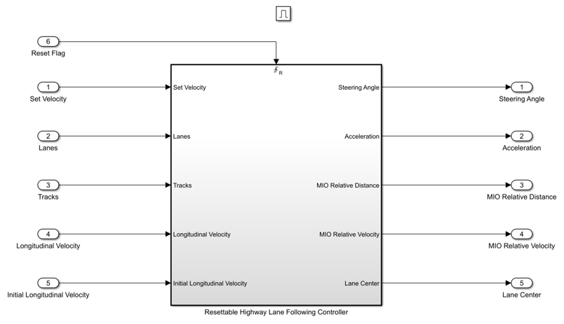
The enabled subsystem contains a resettable subsystem. The resettable subsystem resets the lane following controller to its default state when Reset Flag is set. Open the Resettable Highway Lane Following Controller subsystem.
open_system("RTHLFControllerTarget/Highway Lane Following Controller/Resettable Highway Lane Following Controller")
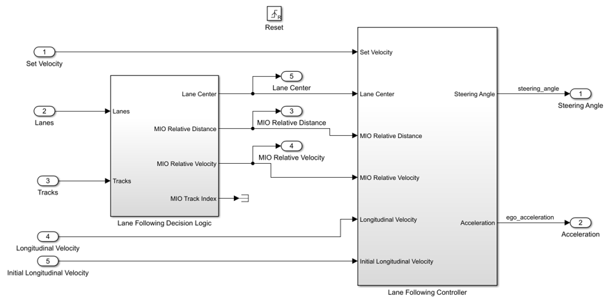
This subsystem is a combination of the Lane Following Decision Logic and Lane Following Controller subsystems. These subsystems are similar to the ones used in the Generate Code for Highway Lane Following Controller example.
Deploy Target Model
Follow these steps to deploy the model to a real-time machine.
1. Configure the UDP blocks in the host and target models.
The UDP Send and UDP Receive blocks used in the host and target models require valid IP addresses for the host and target machines. This example ships with the helperSLRTUDPSetup.m file, which updates these blocks with your specified IP addresses. You can update these blocks manually, or by using the helperSLRTUDPSetup function as shown:
% Specify host model and IP address of Host machine
hostMdl = "RTHLFControllerHost";
hostIP = "10.1.10.16";
% Specify Target model and IP address of Target machine
targetMdl = "RTHLFControllerTarget";
targetIP = "10.1.10.15";
% Invoke the function to update the blocks
helperSLRTUDPSetup(targetMdl,targetIP,hostMdl,hostIP);
2. Connect to the target machine.
Connect to the target machine by defining an slrealtime object to manage the target computer.
% Create slrealtime object
tg = slrealtime;
% Specify IP address for target machine
setipaddr(tg,'10.1.10.15')
% Connect to target
connect(tg);
The real-time operating system (RTOS) version on the target computer must match with that on the host computer. Otherwise, you cannot connect to the target computer. Run the update(tg) command to update the RTOS version on the target computer.
3. Update SystemTargetFile configuration parameter and build the target model, which generates an slrealtime application file, RTHLFControllerTarget.mldatx.
% Read the system target file for the target
modelSTF = getSTFName(tg);
% Set SystemTargetFile parameter in the target model
set_param(targetMdl,"SystemTargetFile",modelSTF);
save_system(targetMdl);
% Build the target model
slbuild(targetMdl);
4. Load the real-time application to the target.
Load the generated RTHLFControllerTarget.mldax application to the target machine.
% Load the controller model to the target
load(tg,targetMdl);
5. Execute the real-time application on the target.
% Start the loaded application on the target machine.
start(tg);
Alternatively, you can deploy the target model by using the Simulink graphical user interface.
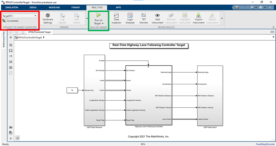
On the Real-Time tab, in the Connect To Target Computer section, select your target machine from the list. Use the slrtExplorer (Simulink Real-Time) to configure the target.
To deploy and run the controller model on the target machine, select Run on Target.
Simulate Host Model and Visualize Results
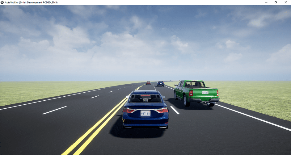
Configure the RTHLFControllerHost model to simulate the scenario_LFACC_03_Curve_StopnGo scenario. This scenario contains six vehicles, including the ego vehicle, and defines their trajectories.
helperSLHLFControllerHostSetup(scenarioFcnName="scenario_LFACC_03_Curve_StopnGo");
Simulate the host model.
sim(hostMdl);
Stop and unload the application in the target machine.
stop(tg);
Plot the performance metrics for the lateral controller.
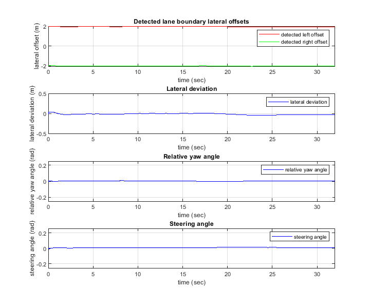
hFigLatResults = helperPlotLFLateralResults(logsout);
Examine the results.
The Detected lane boundary lateral offsets plot shows the lateral offsets of the detected left-lane and right-lane boundaries from the center of the lane. This signal is input to the controller.
The Lateral deviation plot shows the lateral deviation of the ego vehicle from the centerline of the lane. Ideally, lateral deviation is zero meters, which implies that the ego vehicle exactly follows the centerline. Small deviations occur when the vehicle changes velocity to avoid collision with another vehicle. This signal is input to the controller.
The Relative yaw angle plot shows the relative yaw angle between the ego vehicle and the centerline of the lane. The relative yaw angle is close to zero radians, which implies that the heading angle of the ego vehicle closely matches the yaw angle of the centerline. This signal is input to the controller.
The Steering angle plot shows the steering angle of the ego vehicle. Observe that the plot shows little deviation, indicating that the steering angle trajectory is smooth. This signal is output by the controller.
Close the figure.
close(hFigLatResults);
Plot the performance metrics for the longitudinal controller.
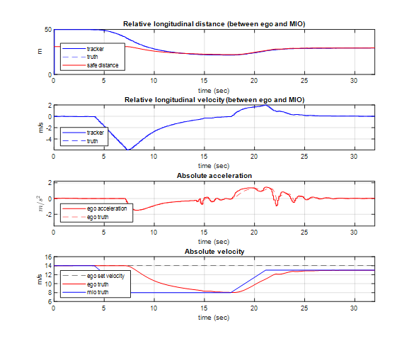
hFigLongResults = helperPlotLFLongitudinalResults(logsout,time_gap,default_spacing);
Examine the results.
The Relative longitudinal distance plot shows the distance between the ego vehicle and the MIO. In this case, the ego vehicle approaches the MIO and even exceeds the safe distance, in some cases. This signal is input to the controller.
The Relative longitudinal velocity plot shows the relative velocity between the ego vehicle and the MIO. Because this example contains no tracker and tracks data filled using ground truth, the estimated velocity is almost identical to the ground truth. This signal is input to the controller.
The Absolute acceleration plot shows that the controller commands the vehicle to decelerate when it approaches the MIO. This signal is output by the controller.
The Absolute velocity plot shows the ego vehicle initially follows the set velocity, but avoids a collision by slowing down when the MIO slows down. This signal is input to the controller.
Close the figure.
close(hFigLongResults);
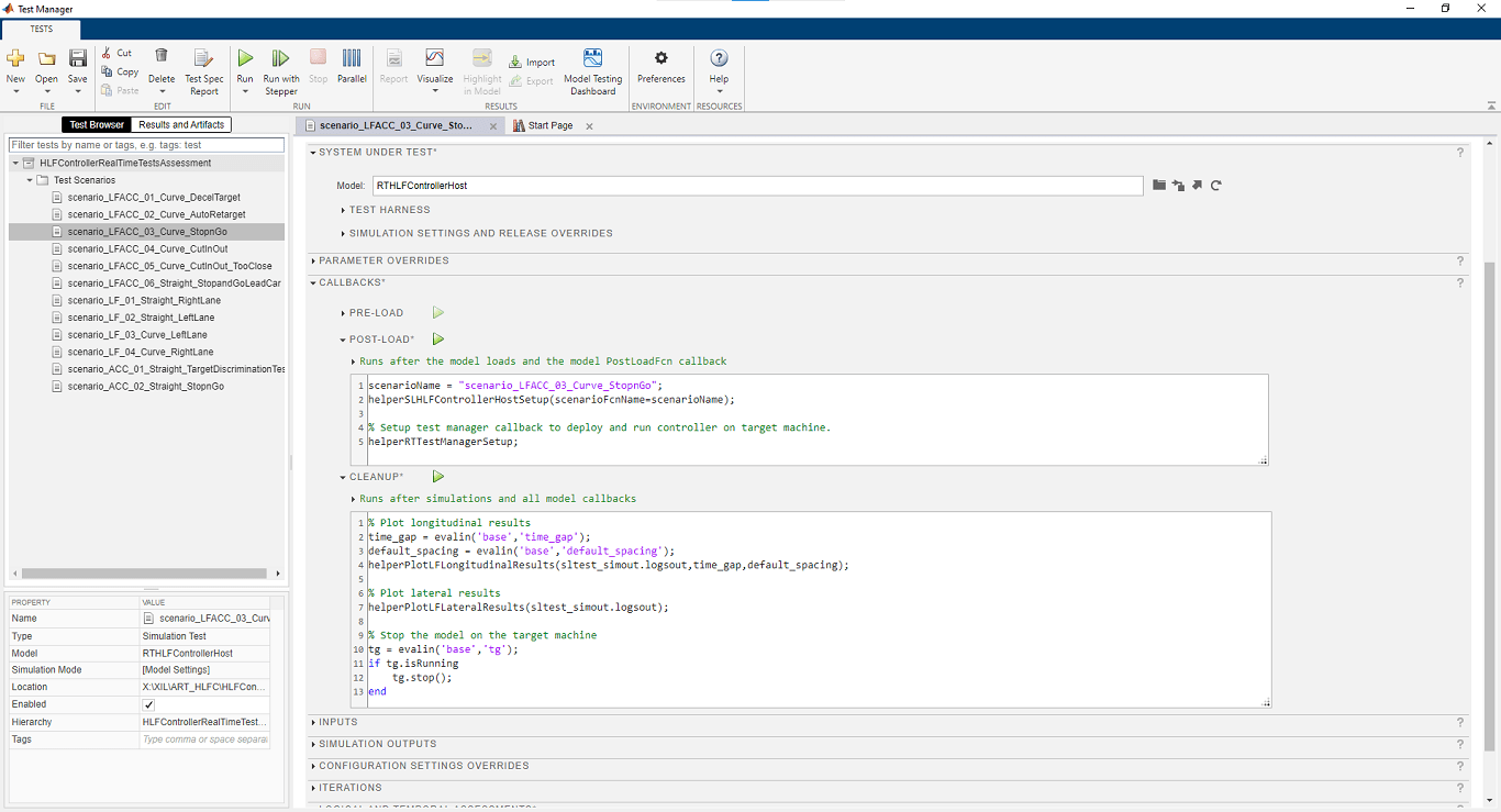
Explore Test Manager File
Simulink Test includes the Test Manager, which you can use to author test cases for Simulink models. After authoring your test cases, you can group them and execute them individually or in a batch.
This example reuses the test scenarios from the Automate Testing for Highway Lane Following Controller example.
This example uses SETUP callback of the test file to build the target application and create or read an slreatime object, which you can use in the callbacks of each test case.
Open the test file HLFControllerRealTimeTestsAssessment.mldatx in the Test Manager and explore the configuration.
sltestmgr
sltest.testmanager.load("HLFControllerRealTimeTestsAssessment.mldatx");
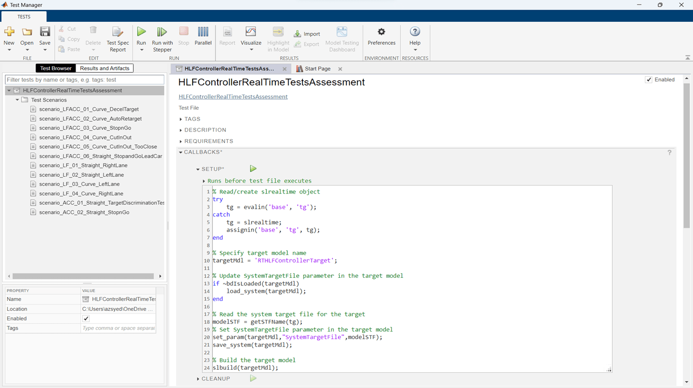
You can also run individual test scenarios using these test case callbacks:
The POST-LOAD callback calls the
helperRTTestManagerSetupto configure the target model to deploy and run on a real-time machine. It also configures the host model for a test scenario.The CLEANUP callback stops the model running on target and calls the functions,
helperPlotLFLongitudinalResultsandhelperPlotLFLateralResultsto plot the results of the simulation run.
Automate Testing
Using the created Test Manager file, run a single test case to test the application on a real-time machine.
Running the test scenarios from test file requires a connection with the target machine. If the target machine is not already connected, refer to steps 1–3 of the Deploy Target Model section.
Use this code to test the lane following controller model with the scenario_LFACC_03_Curve_StopnGo test scenario from Simulink Test.
testFile = sltest.testmanager.load("HLFControllerRealTimeTestsAssessment.mldatx");
testSuite = getTestSuiteByName(testFile,"Test Scenarios");
testCase = getTestCaseByName(testSuite,"scenario_LFACC_03_Curve_StopnGo");
resultObj = run(testCase);
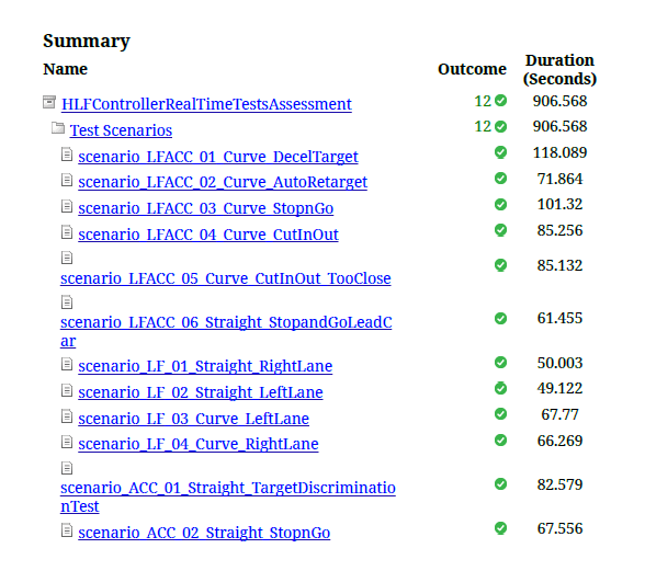
To generate a report after the simulation, use this code:
sltest.testmanager.report(resultObj,"Report.pdf", ...
Title="Real-Time Highway Lane Following Controller Test Assessment", ...
IncludeMATLABFigures=true, ...
IncludeErrorMessages=true, ...
IncludeTestResults=false, ...
LaunchReport=true);
Examine Report.pdf. Observe that the Test Environment section shows the platform on which the test is run and the MATLAB version used for testing. The Summary section shows the outcome of the test and the duration of the simulation in seconds. The Results section shows pass or fail results based on the assessment criteria. This section also shows the logged plots from the CLEANUP callback commands.
Run and Explore Results for All Test Scenarios
You can simulate the system for all the tests by using run(testFile). Alternatively, you can simulate the system by clicking Play in the Test Manager.
When the test simulations are complete, you can view the results for all the tests in the Results and Artifacts tab of the Test Manager. For each test case, the Check Static Range (Simulink) blocks in the model are associated with the Test Manager to visualize overall pass or fail results.
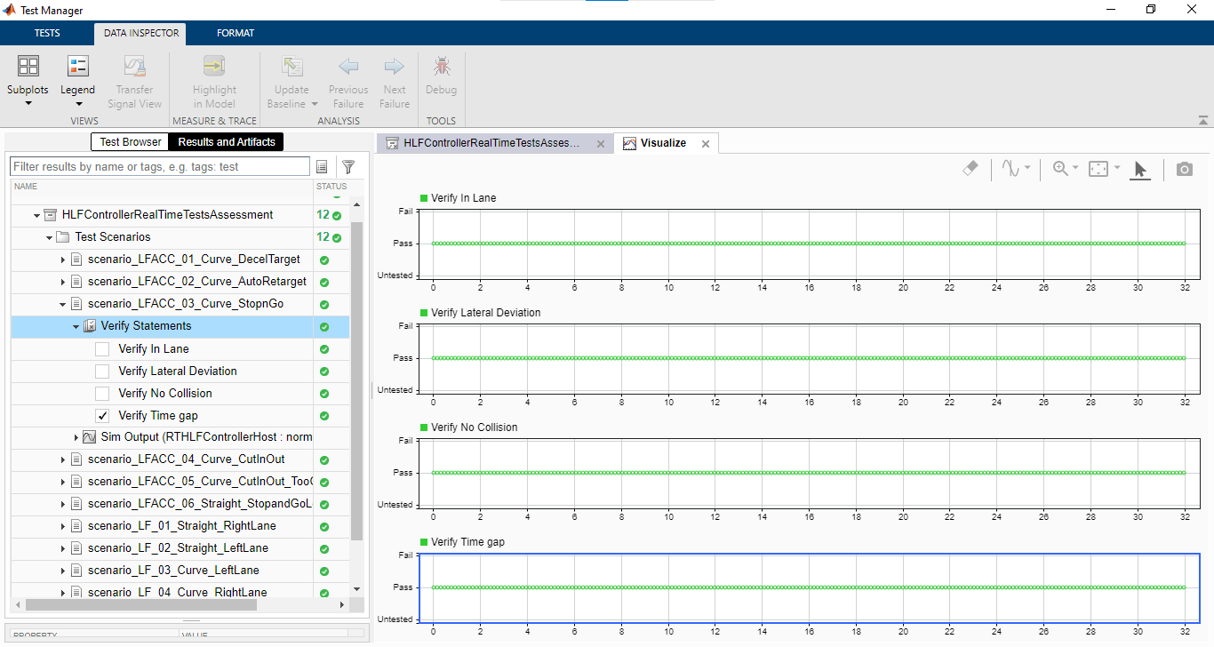
You can find the generated report in the current working directory. This report contains a detailed summary of the pass or fail statuses and plots for each test case.
See Also
Blocks
- Scenario Reader | Simulation 3D Scene Configuration | UDP Send (Simulink Real-Time) | UDP Receive (Simulink Real-Time) | Byte Unpacking (Simulink Real-Time) | Byte Packing (Simulink Real-Time)
Topics
- Automate Real-Time Testing for Forward Vehicle Sensor Fusion
- Automate Real-Time Testing of Highway Lane Following Controller Using ASAM XIL
- Generate Code for Highway Lane Following Controller
- Automate Testing for Highway Lane Following Controller
- Automate Testing for Highway Lane Following Controls and Sensor Fusion
- Lane Following Control with Sensor Fusion and Lane Detection
- Highway Lane Following