Solve PDE Using Physics-Informed Neural Network

This example uses:

This example shows how to train a physics-informed neural network (PINN) to predict the solutions of an partial differential equation (PDE).

A physics-informed neural network (PINN) [1] is a neural network that incorporates physical laws into its structure and training process. For example, you can train a neural network that outputs the solution of a PDE that defines a physical system.

This example trains a PINN that takes samples $(x, t)$ as input and outputs $u (x, t)$ , where $u$ is the solution of the Burger's equation:

$\frac{\partial u}{\partial t} + u \frac{\partial u}{\partial x} - \frac{0.01}{π} \frac{\partial^{2} u}{\partial x^{2}} = 0,$

with $u (x, 0) = - s i n (π x)$ as the initial condition, and $u (- 1, t) = 0$ and $u (1, t) = 0$ as the boundary conditions.

This diagram illustrates the flow of data through the PINN.

Diagram of the data flow of the neural network. The input is x_1, x_2, ... x_N, and t. The output is the PDE solution u(x,t).

Training this model does not require collecting data in advance. You can generate data using the definition of the PDE and the constraints.

Generate Training Data

Training the model requires a data set of collocation points that enforce the boundary conditions, enforce the initial conditions, and fulfill the Burger's equation.

Select 25 equally spaced time points to enforce each of the boundary conditions $u (- 1, t) = 0$ and $u (1, t) = 0$ .

numBoundaryConditionPoints = [25 25];

x0BC1 = -1*ones(1,numBoundaryConditionPoints(1));
x0BC2 = ones(1,numBoundaryConditionPoints(2));

t0BC1 = linspace(0,1,numBoundaryConditionPoints(1));
t0BC2 = linspace(0,1,numBoundaryConditionPoints(2));

u0BC1 = zeros(1,numBoundaryConditionPoints(1));
u0BC2 = zeros(1,numBoundaryConditionPoints(2));

Select 50 equally spaced spatial points to enforce the initial condition $u (x, 0) = - s i n (π x)$ .

numInitialConditionPoints  = 50;

x0IC = linspace(-1,1,numInitialConditionPoints);
t0IC = zeros(1,numInitialConditionPoints);
u0IC = -sin(pi*x0IC);

Group together the data for initial and boundary conditions.

X0 = [x0IC x0BC1 x0BC2];
T0 = [t0IC t0BC1 t0BC2];
U0 = [u0IC u0BC1 u0BC2];

Uniformly sample 10,000 points $(t, x) \in (0, 1) \times (- 1, 1)$ to enforce the output of the network to fulfill the Burger's equation.

numInternalCollocationPoints = 10000;

points = rand(numInternalCollocationPoints,2);

dataX = 2*points(:,1)-1;
dataT = points(:,2);

Define Neural Network Architecture

Define a multilayer perceptron neural network architecture.

Diagram of the neual network architecture. The layers are connected in series. The input is passed through 8 fully connected layers that are each proceeded by a tanh layer. The output of the final tanh layer is connected to a fully connected layer, which outputs the network predictions.

For the repeated fully connected layers, specify an output size of 20.
For the final fully connected layer, specify an output size of 1.

Specify the network hyperparameters.

numBlocks = 8;
fcOutputSize = 20;

Create the neural network. To easily construct a neural network with repeating blocks of layers, you can repeat blocks of layers using the repmat function.

fcBlock = [
    fullyConnectedLayer(fcOutputSize)
    tanhLayer];

layers = [
    featureInputLayer(2)
    repmat(fcBlock,[numBlocks 1])
    fullyConnectedLayer(1)]

layers = 
  18×1 Layer array with layers:

     1   ''   Feature Input     2 features
     2   ''   Fully Connected   20 fully connected layer
     3   ''   Tanh              Hyperbolic tangent
     4   ''   Fully Connected   20 fully connected layer
     5   ''   Tanh              Hyperbolic tangent
     6   ''   Fully Connected   20 fully connected layer
     7   ''   Tanh              Hyperbolic tangent
     8   ''   Fully Connected   20 fully connected layer
     9   ''   Tanh              Hyperbolic tangent
    10   ''   Fully Connected   20 fully connected layer
    11   ''   Tanh              Hyperbolic tangent
    12   ''   Fully Connected   20 fully connected layer
    13   ''   Tanh              Hyperbolic tangent
    14   ''   Fully Connected   20 fully connected layer
    15   ''   Tanh              Hyperbolic tangent
    16   ''   Fully Connected   20 fully connected layer
    17   ''   Tanh              Hyperbolic tangent
    18   ''   Fully Connected   1 fully connected layer

Convert the layer array to a dlnetwork object.

net = dlnetwork(layers)

net = 
  dlnetwork with properties:

         Layers: [18×1 nnet.cnn.layer.Layer]
    Connections: [17×2 table]
     Learnables: [18×3 table]
          State: [0×3 table]
     InputNames: {'input'}
    OutputNames: {'fc_9'}
    Initialized: 1

  View summary with summary.

Training a PINN can result in better accuracy when the learnable parameters have data type double. Convert the network learnables to double using the dlupdate function. Note that not all neural networks support learnables of type double, for example, networks that use GPU optimizations that rely on learnables with type single.

net = dlupdate(@double,net);

Define Model Loss Function

Create the function modelLoss that takes as input the neural network, the network inputs, and the initial and boundary conditions, and returns the gradients of the loss with respect to the learnable parameters and the corresponding loss.

The model is trained by enforcing that given an input $(x, t)$ the output of the network $u (x, t)$ fulfills the Burger's equation, the boundary conditions, and the initial condition. In particular, two quantities contribute to the loss to be minimized:

$loss = {MSE}_{f} + {MSE}_{u}$ ,

where ${MSE}_{f} = \frac{1}{N_{f}} \sum_{i = 1}^{N_{f}} {| f (x_{f}^{i}, t_{f}^{i}) |}^{2}$ , ${MSE}_{u} = \frac{1}{N_{u}} \sum_{i = 1}^{N_{u}} {| u (x_{u}^{i}, t_{u}^{i}) - u^{i} |}^{2}$ , the function $f$ is the left-hand side of the Burger's equation, and ${x_{u}^{i}, t_{u}^{i}}_{i = 1}^{N_{u}}$ correspond to collocation points on the boundary of the computational domain and account for both boundary and initial condition, and ${x_{f}^{i}, t_{f}^{i}}_{i = 1}^{N_{f}}$ are points in the interior of the domain.

function [loss,gradients] = modelLoss(net,X,T,X0,T0,U0)

% Make predictions with the initial conditions.
XT = cat(1,X,T);
U = forward(net,XT);

% Calculate derivatives with respect to X and T.
X = stripdims(X);
T = stripdims(T);
U = stripdims(U);
Ux = dljacobian(U,X,1);
Ut = dljacobian(U,T,1);

% Calculate second-order derivatives with respect to X.
Uxx = dldivergence(Ux,X,1);

% Calculate mseF. Enforce Burger's equation.
f = Ut + U.*Ux - (0.01./pi).*Uxx;
mseF = mean(f.^2);

% Calculate mseU. Enforce initial and boundary conditions.
XT0 = cat(1,X0,T0);
U0Pred = forward(net,XT0);
mseU = l2loss(U0Pred,U0);

% Calculated loss to be minimized by combining errors.
loss = mseF + mseU;

% Calculate gradients with respect to the learnable parameters.
gradients = dlgradient(loss,net.Learnables);

end

Specify Training Options

Specify the training options:

Train using the L-BFGS solver and use the default options for the L-BFGS solver state.
Train for 1500 iterations
Stop training early when the norm of the gradients or steps are smaller than $1 0^{- 5}$ .

solverState = lbfgsState;
maxIterations = 1500;
gradientTolerance = 1e-5;
stepTolerance = 1e-5;

Train Neural Network

Convert the training data to dlarray objects. Specify that the inputs X and T have format "BC" (batch, channel) and that the initial conditions have format "CB" (channel, batch).

X = dlarray(dataX,"BC");
T = dlarray(dataT,"BC");
X0 = dlarray(X0,"CB");
T0 = dlarray(T0,"CB");
U0 = dlarray(U0,"CB");

Accelerate the loss function using the dlaccelerate function. For more information about function acceleration, see Deep Learning Function Acceleration for Custom Training Loops.

accfun = dlaccelerate(@modelLoss);

Create a function handle containing the loss function for the L-BFGS update step. In order to evaluate the dlgradient function inside the modelLoss function using automatic differentiation, use the dlfeval function.

lossFcn = @(net) dlfeval(accfun,net,X,T,X0,T0,U0);

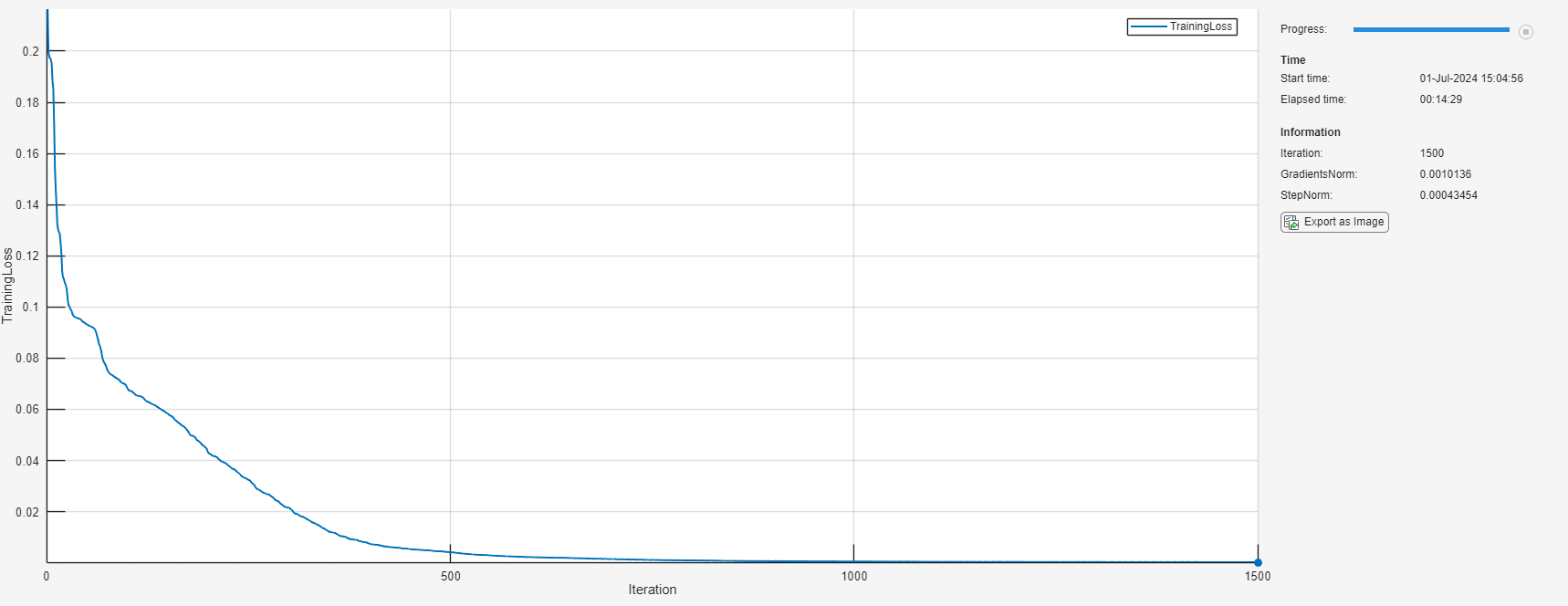
Initialize the TrainingProgressMonitor object. At each iteration, plot the loss and monitor the norm of the gradients and steps. Because the timer starts when you create the monitor object, make sure that you create the object close to the training loop.

monitor = trainingProgressMonitor( ...
    Metrics="TrainingLoss", ...
    Info=["Iteration" "GradientsNorm" "StepNorm"], ...
    XLabel="Iteration");

Train the network using a custom training loop using the full data set at each iteration. For each iteration:

Update the network learnable parameters and solver state using the lbfgsupdate function.
Update the training progress monitor.
Stop training early if the norm of the gradients are less the specified tolerances or if the line search fails.

iteration = 0;
while iteration < maxIterations && ~monitor.Stop
    iteration = iteration + 1;
    [net, solverState] = lbfgsupdate(net,lossFcn,solverState);

    updateInfo(monitor, ...
        Iteration=iteration, ...
        GradientsNorm=solverState.GradientsNorm, ...
        StepNorm=solverState.StepNorm);

    recordMetrics(monitor,iteration,TrainingLoss=solverState.Loss);

    monitor.Progress = 100*iteration/maxIterations;

    if solverState.GradientsNorm < gradientTolerance || ...
            solverState.StepNorm < stepTolerance || ...
            solverState.LineSearchStatus == "failed"
        break
    end

end

Evaluate Model Accuracy

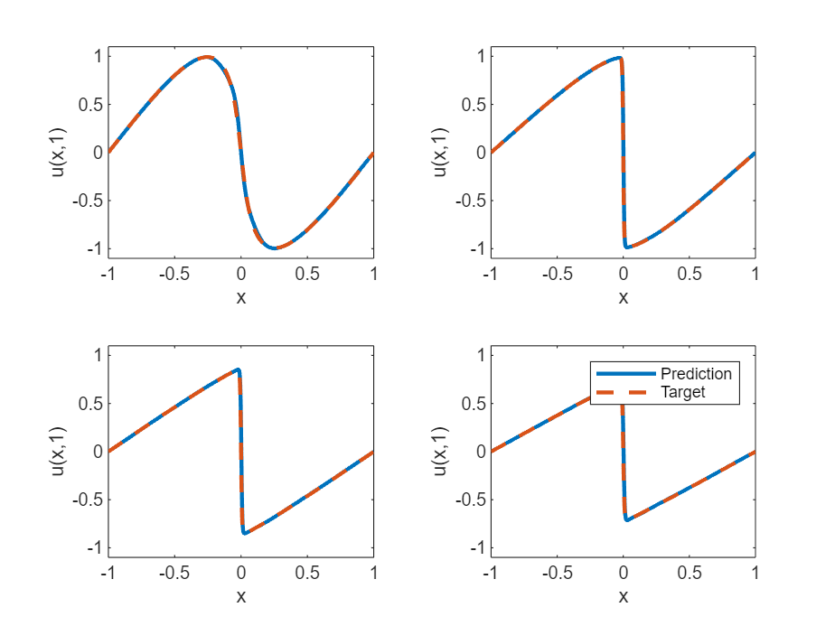
For values of $t$ at 0.25, 0.5, 0.75, and 1, compare the predicted values of the deep learning model with the true solutions of the Burger's equation.

Set the target times to test the model at. For each time, calculate the solution at 1001 equally spaced points in the range [-1,1].

tTest = [0.25 0.5 0.75 1];
numObservationsTest = numel(tTest);

szXTest = 1001;
XTest = linspace(-1,1,szXTest);
XTest = dlarray(XTest,"CB");

Test the model. For each of the test inputs, predict the PDE solutions using the PINN and compare them to the solutions given by the solveBurgers function, listed in the Solve Burger's Equation Function section of the example. To access this function, open the example as a live script. Evaluate the accuracy by computing the relative error between the predictions and targets.

UPred = zeros(numObservationsTest,szXTest);
UTest = zeros(numObservationsTest,szXTest);

for i = 1:numObservationsTest
    t = tTest(i);

    TTest = repmat(t,[1 szXTest]);
    TTest = dlarray(TTest,"CB");
    XTTest = cat(1,XTest,TTest);

    UPred(i,:) = forward(net,XTTest);
    UTest(i,:) = solveBurgers(extractdata(XTest),t,0.01/pi);
end

err = norm(UPred - UTest) / norm(UTest)

err = 
0.0237

Visualize the test predictions in a plot.

figure
tiledlayout("flow")

for i = 1:numel(tTest)
    nexttile
    
    plot(XTest,UPred(i,:),"-",LineWidth=2);

    hold on
    plot(XTest, UTest(i,:),"--",LineWidth=2)
    hold off

    ylim([-1.1, 1.1])
    xlabel("x")
    ylabel("u(x," + t + ")")
end

legend(["Prediction" "Target"])

Solve Burger's Equation Function

The solveBurgers function returns the true solution of Burger's equation at times t as outlined in [2].

function U = solveBurgers(X,t,nu)

% Define functions.
f = @(y) exp(-cos(pi*y)/(2*pi*nu));
g = @(y) exp(-(y.^2)/(4*nu*t));

% Initialize solutions.
U = zeros(size(X));

% Loop over x values.
for i = 1:numel(X)
    x = X(i);

    % Calculate the solutions using the integral function. The boundary
    % conditions in x = -1 and x = 1 are known, so leave 0 as they are
    % given by initialization of U.
    if abs(x) ~= 1
        fun = @(eta) sin(pi*(x-eta)) .* f(x-eta) .* g(eta);
        uxt = -integral(fun,-inf,inf);
        fun = @(eta) f(x-eta) .* g(eta);
        U(i) = uxt / integral(fun,-inf,inf);
    end
end

end

References

Maziar Raissi, Paris Perdikaris, and George Em Karniadakis, Physics Informed Deep Learning (Part I): Data-driven Solutions of Nonlinear Partial Differential Equations https://arxiv.org/abs/1711.10561
C. Basdevant, M. Deville, P. Haldenwang, J. Lacroix, J. Ouazzani, R. Peyret, P. Orlandi, A. Patera, Spectral and finite difference solutions of the Burgers equation, Computers & fluids 14 (1986) 23–41.