Pattern Recognition with a Shallow Neural Network
In addition to function fitting, neural networks are also good at recognizing patterns.
For example, suppose you want to classify a tumor as benign or malignant, based on uniformity of cell size, clump thickness, mitosis, etc. You have 699 example cases for which you have 9 features and the correct classification as benign or malignant.
As with function fitting, there are two ways to solve this problem:
Use the Neural Net Pattern Recognition app, as described in Pattern Recognition Using the Neural Net Pattern Recognition App.
Use command-line functions, as described in Pattern Recognition Using Command-Line Functions.
It is generally best to start with the app, and then use the app to automatically generate command-line scripts. Before using either method, first define the problem by selecting a data set. Each of the neural network apps has access to many sample data sets that you can use to experiment with the toolbox (see Sample Data Sets for Shallow Neural Networks). If you have a specific problem that you want to solve, you can load your own data into the workspace. The next section describes the data format.
Tip
To interactively build and visualize deep learning neural networks, use the Deep Network Designer app. For more information, see Get Started with Deep Network Designer.
Defining a Problem
To define a pattern recognition problem, arrange a set of input vectors (predictors) as columns in a matrix. Then arrange another set of response vectors indicating the classes to which the observations are assigned.
When there are only two classes, each response has two elements, 0 and 1, indicating which class the corresponding observation belongs to. For example, you can define a two-class classification problem as follows:
predictors = [7 10 3 1 6; 5 8 1 1 6; 6 7 1 1 6];
responses = [0 0 1 1 0; 1 1 0 0 1];
When predictors are to be classified into N different classes, the responses have N elements. For each response, one element is 1 and the others are 0. For example, the following lines show how to define a classification problem that divides the corners of a 5-by-5-by-5 cube into three classes:
The origin (the first input vector) in one class
The corner farthest from the origin (the last input vector) in a second class
All other points in a third class
predictors  = [0 0 0 0 5 5 5 5; 0 0 5 5 0 0 5 5; 0 5 0 5 0 5 0 5];
responses = [1 0 0 0 0 0 0 0; 0 1 1 1 1 1 1 0; 0 0 0 0 0 0 0 1];
The next section shows how to train a network to recognize patterns, using the Neural Net Pattern Recognition app. This example uses an example data set provided with the toolbox.
Pattern Recognition Using the Neural Net Pattern Recognition App
This example shows how to train a shallow neural network to classify patterns using the Neural Net Pattern Recognition app.
Open the Neural Net Pattern Recognition app using nprtool.
nprtool
Select Data
The Neural Net Pattern Recognition app has example data to help you get started training a neural network.
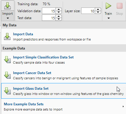
To import example glass classification data, select Import > Import Glass Data Set. You can use this data set to train a neural network to classify glass as window or non-window, using properties of the glass chemistry. If you import your own data from file or the workspace, you must specify the predictors and responses, and whether the observations are in rows or columns.
Information about the imported data appears in the Model Summary. This data set contains 214 observations, each with 9 features. Each observation is classified into one of two classes: window or non-window.

Split the data into training, validation, and test sets. Keep the default settings. The data is split into:
70% for training.
15% to validate that the network is generalizing and to stop training before overfitting.
15% to independently test network generalization.
For more information on data division, see Divide Data for Optimal Neural Network Training.
Create Network
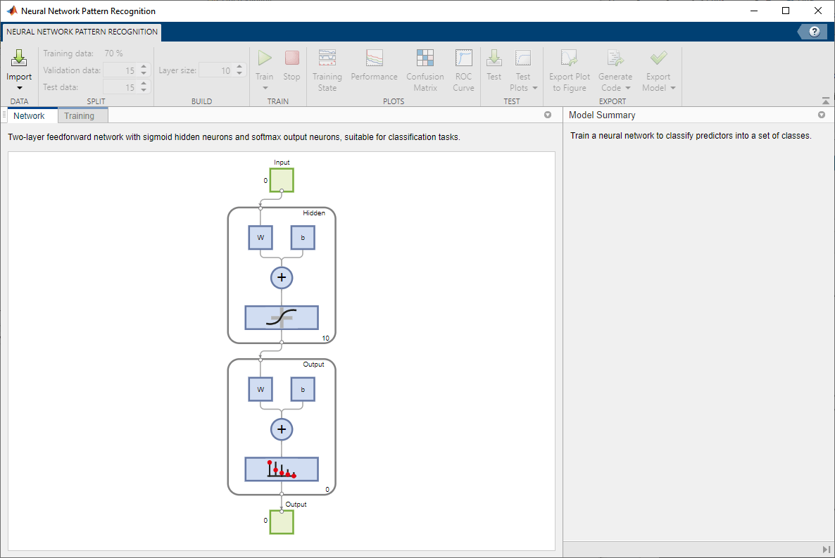
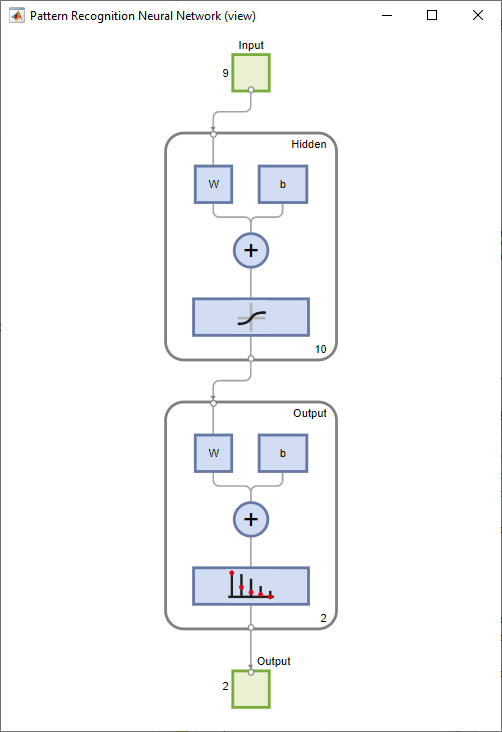
The network is a two-layer feedforward network with a sigmoid transfer function in the hidden layer and a softmax transfer function in the output layer. The size of the hidden layer corresponds to the number of hidden neurons. The default layer size is 10. You can see the network architecture in the Network pane. The number of output neurons is set to 2, which is equal to the number of classes specified by the response data.

Train Network
To train the network, click Train.
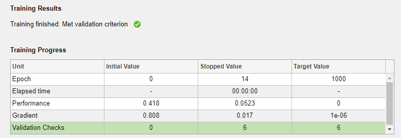
In the Training pane, you can see the training progress. Training continues until one of the stopping criteria is met. In this example, training continues until the validation error is larger than or equal to the previously smallest validation error for six consecutive validation iterations ("Met validation criterion").
Analyze Results
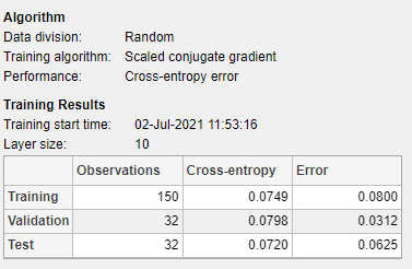
The Model Summary contains information about the training algorithm and the training results for each data set.
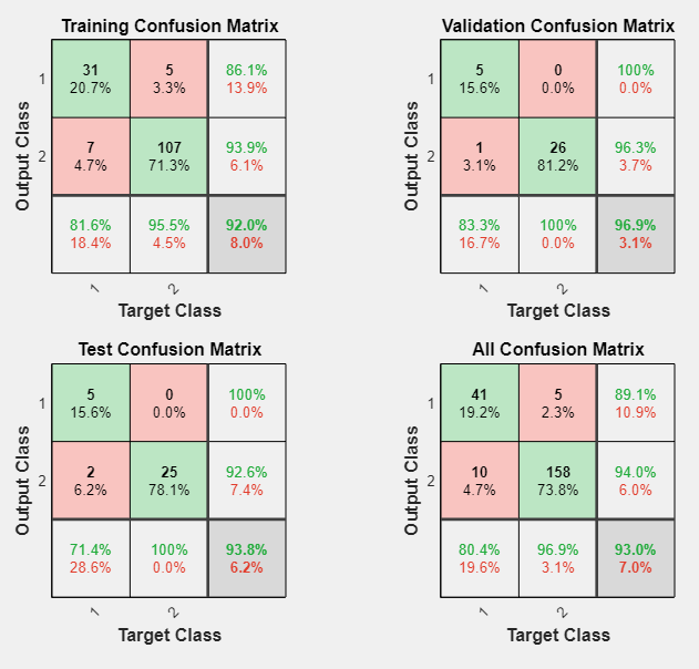
You can further analyze the results by generating plots. To plot the confusion matrices, in the Plots section, click Confusion Matrix. The network outputs are very accurate, as you can see by the high numbers of correct classifications in the green squares (diagonal) and the low numbers of incorrect classifications in the red squares (off-diagonal).
View the ROC curve to obtain additional verification of network performance. In the Plots section, click ROC Curve.
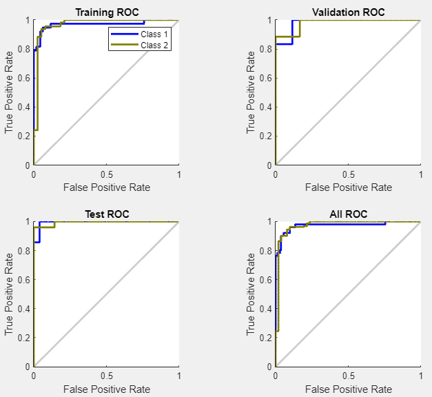
The colored lines in each axis represent the ROC curves. The ROC curve is a plot of the true positive rate (sensitivity) versus the false positive rate (1 - specificity) as the threshold is varied. A perfect test would show points in the upper-left corner, with 100% sensitivity and 100% specificity. For this problem, the network performs very well.
If you are unhappy with the network performance, you can do one of the following:
Train the network again.
Increase the number of hidden neurons.
Use a larger training data set.
If performance on the training set is good but the test set performance is poor, this could indicate the model is overfitting. Reducing the number of neurons can reduce the overfitting.
You can also evaluate the network performance on an additional test set. To load additional test data to evaluate the network with, in the Test section, click Test. The Model Summary displays the additional test results. You can also generate plots to analyze the additional test results.
Generate Code
Select Generate Code > Generate Simple Training Script to create MATLAB code to reproduce the previous steps from the command line. Creating MATLAB code can be helpful if you want to learn how to use the command line functionality of the toolbox to customize the training process. In Pattern Recognition Using Command-Line Functions, you will investigate the generated scripts in more detail.

Export Network
You can export your trained network to the workspace or Simulink®. You can also deploy the network with MATLAB Compiler™ and other MATLAB code generation tools. To export your trained network and results, select Export Model > Export to Workspace.

Pattern Recognition Using Command-Line Functions
The easiest way to learn how to use the command-line functionality of the toolbox is to generate scripts from the apps, and then modify them to customize the network training. As an example, look at the simple script that was created in the previous section using the Neural Net Pattern Recognition app.
% Solve a Pattern Recognition Problem with a Neural Network
% Script generated by Neural Pattern Recognition app
% Created 22-Mar-2021 16:50:20
%
% This script assumes these variables are defined:
%
%   glassInputs - input data.
%   glassTargets - target data.

x = glassInputs;
t = glassTargets;

% Choose a Training Function
% For a list of all training functions type: help nntrain
% 'trainlm' is usually fastest.
% 'trainbr' takes longer but may be better for challenging problems.
% 'trainscg' uses less memory. Suitable in low memory situations.
trainFcn = 'trainscg';  % Scaled conjugate gradient backpropagation.

% Create a Pattern Recognition Network
hiddenLayerSize = 10;
net = patternnet(hiddenLayerSize, trainFcn);

% Setup Division of Data for Training, Validation, Testing
net.divideParam.trainRatio = 70/100;
net.divideParam.valRatio = 15/100;
net.divideParam.testRatio = 15/100;

% Train the Network
[net,tr] = train(net,x,t);

% Test the Network
y = net(x);
e = gsubtract(t,y);
performance = perform(net,t,y)
tind = vec2ind(t);
yind = vec2ind(y);
percentErrors = sum(tind ~= yind)/numel(tind);

% View the Network
view(net)

% Plots
% Uncomment these lines to enable various plots.
%figure, plotperform(tr)
%figure, plottrainstate(tr)
%figure, ploterrhist(e)
%figure, plotconfusion(t,y)
%figure, plotroc(t,y)
You can save the script and then run it from the command line to reproduce the results of the previous training session. You can also edit the script to customize the training process. In this case, follow each step in the script.
Select Data
The script assumes that the predictor and response vectors are already loaded into the workspace. If the data is not loaded, you can load it as follows:
load glass_datasetglassInputs and the responses
glassTargets into the workspace.This data set is one of the sample data sets that is part of the toolbox. For
information about the data sets available, see Sample Data Sets for Shallow Neural Networks. You can
also see a list of all available data sets by entering the command help
nndatasets. You can load the variables from any of these data sets using your
own variable names. For example, the
command
[x,t] = glass_dataset;
x and the glass responses into
the array t.Choose Training Algorithm
Define training algorithm.
trainFcn = 'trainscg'; % Scaled conjugate gradient backpropagation.
Create Network
Create the network. The default network for pattern recognition
(classification) problems, patternnet, is a feedforward network with
the default sigmoid transfer function in the hidden layer, and a softmax transfer function
in the output layer. The network has a single hidden layer with ten neurons
(default).
The network has two output neurons, because there are two response values (classes) associated with each input vector. Each output neuron represents a class. When an input vector of the appropriate class is applied to the network, the corresponding neuron should produce a 1, and the other neurons should output a 0.
hiddenLayerSize = 10;
net = patternnet(hiddenLayerSize, trainFcn);
Note
More neurons require more computation, and they have a tendency to overfit the data
when the number is set too high, but they allow the network to solve more complicated
problems. More layers require more computation, but their use might result in the
network solving complex problems more efficiently. To use more than one hidden layer,
enter the hidden layer sizes as elements of an array in the patternnet command.
Divide Data
Set up the division of data.
net.divideParam.trainRatio = 70/100;
net.divideParam.valRatio = 15/100;
net.divideParam.testRatio = 15/100;
With these settings, the predictor vectors and response vectors are randomly divided, with 70% for training, 15% for validation, and 15% for testing. For more information about the data division process, see Divide Data for Optimal Neural Network Training.
Train Network
Train the network.
[net,tr] = train(net,x,t);
During training, the training progress window opens. You can interrupt training at any
point by clicking the stop button ![]() .
.

Training finished when the validation error was larger than or equal to the previously smallest validation error for six consecutive validation iterations, which occurred at epoch 14.
If you click Performance in the training window, a plot of the training errors, validation errors, and test errors appears, as shown in the following figure.
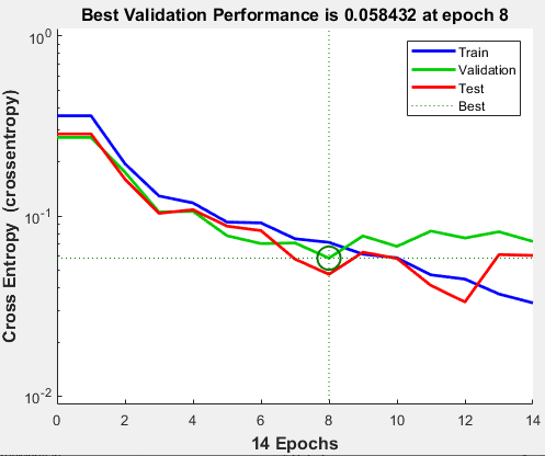
In this example, the result is reasonable as the final cross-entropy error is small.
Test Network
Test the network. After the network has trained, you can use it to compute the network outputs. The following code calculates the network outputs, errors, and overall performance.
y = net(x);
e = gsubtract(t,y);
performance = perform(net,t,y)
performance =

    0.0659
You can also compute the fraction of misclassified observations. In this example, the model has a very low misclassification rate.
tind = vec2ind(t);
yind = vec2ind(y);
percentErrors = sum(tind ~= yind)/numel(tind)
percentErrors =

    0.0514
It is also possible to calculate the network performance only on the test set, by using the testing indices, which are located in the training record.
tInd = tr.testInd;
tstOutputs = net(x(:,tInd));
tstPerform = perform(net,t(tInd),tstOutputs)
tstPerform =

    2.0163
View Network
View the network diagram.
view(net)
Analyze Results
Use the plotconfusion function to plot the confusion matrix. You can also plot the confusion matrix for each of the data sets by clicking
Confusion in the training window.
figure, plotconfusion(t,y)

The diagonal green cells show the number of cases that were correctly classified, and the off-diagonal red cells show the misclassified cases. The results show very good recognition. If you needed even more accurate results, you could try any of the following approaches:
Reset the initial network weights and biases to new values with
initand train again.Increase the number of hidden neurons.
Use a larger training data set.
Increase the number of input values, if more relevant information is available.
Try a different training algorithm (see Training Algorithms).
In this case, the network results are satisfactory, and you can now put the network to use on new input data.
Next Steps
To get more experience in command line operations, here are some tasks you can try:
During training, open a plot window (such as the confusion plot), and watch it animate.
Plot from the command line with functions such as
plotrocandplottrainstate.
Each time a neural network is trained can result in a different solution due to random initial weight and bias values and different divisions of data into training, validation, and test sets. As a result, different neural networks trained on the same problem can give different outputs for the same input. To ensure that a neural network of good accuracy has been found, retrain several times.
There are several other techniques for improving upon initial solutions if higher accuracy is desired. For more information, see Improve Shallow Neural Network Generalization and Avoid Overfitting.
See Also
Neural
Net Fitting | Neural
Net Time Series | Neural
Net Pattern Recognition | Neural
Net Clustering | Deep Network Designer | trainscg