Fit Rational Models
Rational models, sometimes called rational functions, are ratios of polynomials given by
where n is the degree of the numerator polynomial, and m is the degree of the denominator polynomial. Curve Fitting Toolbox™ supports rational models with 0 ≤ n ≤ 5 and 1 ≤ m ≤ 5. The coefficient associated with xm is always 1, which makes the numerator and denominator unique when the polynomial degrees are the same.
Here rationals are described in terms of the degree of the numerator/the degree of the denominator. For example, a quadratic/cubic rational equation is given by
Like polynomials, rationals are often used when a simple empirical model is required. The main advantage of rationals is their flexibility with data that has a complicated structure. The main disadvantage is that they become unstable when the denominator is around 0. For an example that uses rational polynomials of various degrees, see Example: Rational Fit.
Fit Rational Models Interactively
Open the Curve Fitter app by entering
curveFitterat the MATLAB® command line. Alternatively, on the Apps tab, in the Math, Statistics and Optimization group, click Curve Fitter.In the Curve Fitter app, select curve data. On the Curve Fitter tab, in the Data section, click Select Data. In the Select Fitting Data dialog box, select X data and Y data, or just Y data against an index.
Click the arrow in the Fit Type section to open the gallery, and click Rational in the Regression Models group.
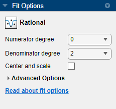
You can specify the following options in the Fit Options pane:
Specify the numerator degree as a nonnegative integer in the range [0 5] and the denominator degree as a positive integer in the range [1 5]. Look in the Results pane to see the model terms, values of the coefficients, and goodness-of-fit statistics.
Optionally, in the Advanced Options section, specify coefficient starting values and constraint bounds, or change algorithm settings. The app calculates random start points for rational models, defined on the interval [0 1]. You can override the start points and specify your own values in the Fit Options pane.
For more information on the settings, see Coefficient Constraints: Specify Bounds and Optimized Start Points.
Selecting a Rational Fit at the Command Line
Specify the model type ratij, where i
is the degree of the numerator polynomial and j is the
degree of the denominator polynomial. For example,
'rat02', 'rat21' or
'rat55'.
For example, to load some data and fit a rational model:
load hahn1;
f = fit( temp, thermex, 'rat32')
plot(f,temp,thermex)
See Example: Rational Fit to fit this example interactively with various rational models.
If you want to modify fit options such as coefficient starting values and
constraint bounds appropriate for your data, or change algorithm settings,
see the table of additional properties with
NonlinearLeastSquares on the fitoptions reference
page.
Example: Rational Fit
This example fits thermal expansion data using a rational fit. The data describes the coefficient of thermal expansion for copper as a function of temperature in kelvin.
A rational fit is defined as the ratio of polynomials given by:
where n is the degree of the numerator polynomial and m is the degree of the denominator polynomial. The rational equations are not associated with physical parameters of the data. Instead, they provide a simple and flexible empirical model that you can use for interpolation and extrapolation.
Load the thermal expansion data in
hahn1. The data set contains a vector of temperatures in kelvin (temp) and a vector of thermal expansion coefficients for copper (thermex).load hahn1Open the Curve Fitter app.
curveFitter
Alternatively, on the Apps tab, in the Math, Statistics and Optimization group, click Curve Fitter.
In the Curve Fitter app, select curve data. On the Curve Fitter tab, in the Data section, click Select Data. In the Select Fitting Data dialog box, specify X data as
tempand Y data asthermex. The Curve Fitter app fits and plots the curve data.Click the arrow in the Fit Type section to open the gallery, and click Rational in the Regression Models group.
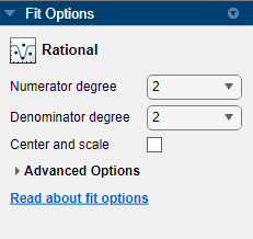
Try a quadratic/quadratic rational fit. In the Fit Options pane, select 2 for both Numerator degree and Denominator degree.
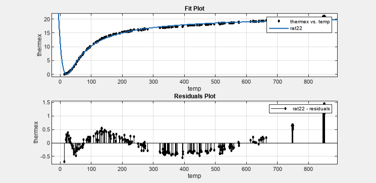
Rename the fit. In the Table Of Fits pane, double-click the Fit Name value and enter
rat22.In the Visualization section, select Residuals Plot. Examine the data, fit, and residuals. Observe that the fit misses the data for the smallest and largest predictor values. Additionally, the residuals show a strong pattern for the entire data set. These observations indicate that a better fit is possible.
Try a cubic/cubic rational fit. First duplicate the current fit. On the Curve Fitter tab, in the File section, click Duplicate. Name the new fit
rat33.In the Fit Options pane, select 3 for both Numerator degree and Denominator degree. Examine the data, fit, and residuals.
Note
Your results depend on random start points and might vary from those shown. The fit can exhibit discontinuities around the zeros of the denominator.
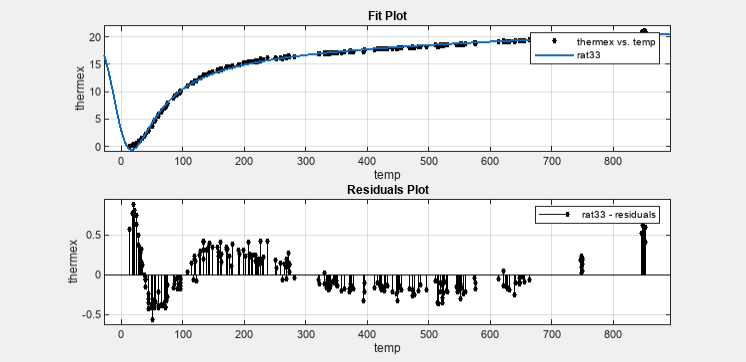
Look at the Results pane. The message and numerical results indicate that the fit did not converge.
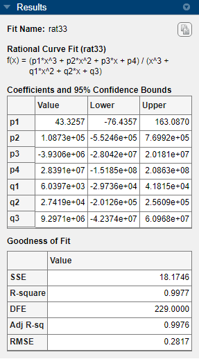
Although the message in the Results pane indicates that you might improve the fit if you increase the maximum number of iterations, a better choice at this stage of the fitting process is to use a different rational equation.
Try a cubic/quadratic rational fit. First duplicate the current fit. On the Curve Fitter tab, in the File section, click Duplicate. Name the new fit
rat32.In the Fit Options pane, select 3 and 2 for Numerator degree and Denominator degree, respectively.
The data variables have very different scales, so select the Center and scale check box. The data, fit, and residuals are shown here.
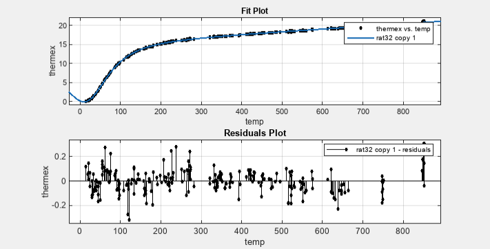
The fit behaves well over the entire data range, and the residuals are randomly scattered about zero. Therefore, you can confidently use this fit for further analysis.
See Also
Apps
Functions
fit|fittype|fitoptions