Main Content

genss

Generalized state-space model

Description

Generalized state-space (genss) models are state-space models that include tunable parameters or components. genss models arise when you combine numeric LTI models with models containing tunable components (control design blocks). For more information about numeric LTI models and control design blocks, see Models with Tunable Coefficients.

You can use generalized state-space models to represent control systems having a mixture of fixed and tunable components. Use generalized state-space models for control design tasks such as parameter studies and parameter tuning with commands such as systune and looptune.

Construction

To construct a genss model:

  • Use series, parallel, lft, or connect, or the arithmetic operators +, -, *, /, \, and ^, to combine numeric LTI models with control design blocks.

  • Use tf or ss with one or more input arguments that is a generalized matrix (genmat) instead of a numeric array

  • Convert any numeric LTI model, control design block, or slTuner (Simulink Control Design) interface (requires Simulink® Control Design™), for example, sys, to genss form using:

    gensys = genss(sys)

    When sys is an slTuner interface, gensys contains all the tunable blocks and analysis points specified in this interface. To compute a tunable model of a particular I/O transfer function, call getIOTransfer(gensys,in,out). Here, in and out are the analysis points of interest. (Use getPoints(sys) to get the full list of analysis points.) Similarly, to compute a tunable model of a particular open-loop transfer function, use getLoopTransfer(gensys,loc). Here, loc is the analysis point of interest.

Properties

Blocks

Structure containing the control design blocks included in the generalized LTI model or generalized matrix. The field names of Blocks are the Name property of each control design block.

You can change some attributes of these control design blocks using dot notation. For example, if the generalized LTI model or generalized matrix M contains a realp tunable parameter a, you can change the current value of a using:

M.Blocks.a.Value = -1;

A,B,C,D

Dependency of state-space matrices on tunable and uncertain parameters, stored as a generalized matrix (genmat), uncertain matrix (umat), or double array.

These properties model the dependency of the state-space matrices on static control design blocks, realp, ureal, ucomplex, or ucomplexm. Dynamic control design blocks such as tunableGain or tunableSS set to their current values, and internal delays are set to zero.

When the corresponding state-space matrix does not depend on any static control design blocks, these properties evaluate to double matrices.

For an example, see Dependence of State-Space Matrices on Parameters.

E

E matrix, stored as a double matrix when the generalized state-space equations are implicit. The value E = [] means that the generalized state-space equations are explicit. For more information about implicit state-space models, see State-Space Models.

StateName

State names, stored as one of the following:

  • Character vector — For first-order models, for example, 'velocity'.

  • Cell array of character vectors — For models with two or more states, for example, {'position';'velocity'}.

  • '' — For unnamed states.

You can assign state names to a genss model only when all its control design blocks are static. Otherwise, specify the state names for the component models before interconnecting them to create the genss model. When you do so, the genss model tracks the assigned state names. For an example, see Track State Names in Generalized State-Space Model.

Default: '' for all states

StateUnit

State unit labels, stored as one of the following:

  • Character vector — For first-order models, for example, 'm/s'.

  • Cell array of character vectors — For models with two or more states, for example, {'m';'m/s'}.

  • '' — For unnamed states.

StateUnit labels the units of each state for convenience, and has no effect on system behavior.

You can assign state units to a genss model only when all its control design blocks are static. Otherwise, specify the state units for the component models before interconnecting them to create the genss model. When you do so, the genss model tracks the assigned state units. For an example, see Track State Names in Generalized State-Space Model.

Default: '' for all states

InternalDelay

Vector storing internal delays.

Internal delays arise, for example, when closing feedback loops on systems with delays, or when connecting delayed systems in series or parallel. For more information about internal delays, see Closing Feedback Loops with Time Delays.

For continuous-time models, internal delays are expressed in the time unit specified by the TimeUnit property of the model. For discrete-time models, internal delays are expressed as integer multiples of the sample time Ts. For example, InternalDelay = 3 means a delay of three sampling periods.

You can modify the values of internal delays. However, the number of entries in sys.InternalDelay cannot change, because it is a structural property of the model.

InputDelay

Input delay for each input channel, specified as a scalar value or numeric vector. For continuous-time systems, specify input delays in the time unit stored in the TimeUnit property. For discrete-time systems, specify input delays in integer multiples of the sample time Ts. For example, InputDelay = 3 means a delay of three sample times.

For a system with Nu inputs, set InputDelay to an Nu-by-1 vector. Each entry of this vector is a numerical value that represents the input delay for the corresponding input channel.

You can also set InputDelay to a scalar value to apply the same delay to all channels.

Default: 0

OutputDelay

Output delays. OutputDelay is a numeric vector specifying a time delay for each output channel. For continuous-time systems, specify output delays in the time unit stored in the TimeUnit property. For discrete-time systems, specify output delays in integer multiples of the sample time Ts. For example, OutputDelay = 3 means a delay of three sampling periods.

For a system with Ny outputs, set OutputDelay to an Ny-by-1 vector, where each entry is a numerical value representing the output delay for the corresponding output channel. You can also set OutputDelay to a scalar value to apply the same delay to all channels.

Default: 0 for all output channels

Ts

Sample time. For continuous-time models, Ts = 0. For discrete-time models, Ts is a positive scalar representing the sampling period. This value is expressed in the unit specified by the TimeUnit property of the model. To denote a discrete-time model with unspecified sample time, set Ts = -1.

Changing this property does not discretize or resample the model.

Default: 0 (continuous time)

TimeUnit

Units for the time variable, the sample time Ts, and any time delays in the model, specified as one of the following values:

  • 'nanoseconds'

  • 'microseconds'

  • 'milliseconds'

  • 'seconds'

  • 'minutes'

  • 'hours'

  • 'days'

  • 'weeks'

  • 'months'

  • 'years'

Changing this property has no effect on other properties, and therefore changes the overall system behavior. Use chgTimeUnit to convert between time units without modifying system behavior.

Default: 'seconds'

InputName

Input channel names, specified as one of the following:

  • Character vector — For single-input models, for example, 'controls'.

  • Cell array of character vectors — For multi-input models.

Alternatively, use automatic vector expansion to assign input names for multi-input models. For example, if sys is a two-input model, enter:

sys.InputName = 'controls';

The input names automatically expand to {'controls(1)';'controls(2)'}.

You can use the shorthand notation u to refer to the InputName property. For example, sys.u is equivalent to sys.InputName.

Input channel names have several uses, including:

  • Identifying channels on model display and plots

  • Extracting subsystems of MIMO systems

  • Specifying connection points when interconnecting models

Default: '' for all input channels

InputUnit

Input channel units, specified as one of the following:

  • Character vector — For single-input models, for example, 'seconds'.

  • Cell array of character vectors — For multi-input models.

Use InputUnit to keep track of input signal units. InputUnit has no effect on system behavior.

Default: '' for all input channels

InputGroup

Input channel groups. The InputGroup property lets you assign the input channels of MIMO systems into groups and refer to each group by name. Specify input groups as a structure. In this structure, field names are the group names, and field values are the input channels belonging to each group. For example:

sys.InputGroup.controls = [1 2];
sys.InputGroup.noise = [3 5];

creates input groups named controls and noise that include input channels 1, 2 and 3, 5, respectively. You can then extract the subsystem from the controls inputs to all outputs using:

sys(:,'controls')

Default: Struct with no fields

OutputName

Output channel names, specified as one of the following:

  • Character vector — For single-output models. For example, 'measurements'.

  • Cell array of character vectors — For multi-output models.

Alternatively, use automatic vector expansion to assign output names for multi-output models. For example, if sys is a two-output model, enter:

sys.OutputName = 'measurements';

The output names automatically expand to {'measurements(1)';'measurements(2)'}.

You can use the shorthand notation y to refer to the OutputName property. For example, sys.y is equivalent to sys.OutputName.

Output channel names have several uses, including:

  • Identifying channels on model display and plots

  • Extracting subsystems of MIMO systems

  • Specifying connection points when interconnecting models

Default: '' for all output channels

OutputUnit

Output channel units, specified as one of the following:

  • Character vector — For single-output models. For example, 'seconds'.

  • Cell array of character vectors — For multi-output models.

Use OutputUnit to keep track of output signal units. OutputUnit has no effect on system behavior.

Default: '' for all output channels

OutputGroup

Output channel groups. The OutputGroup property lets you assign the output channels of MIMO systems into groups and refer to each group by name. Specify output groups as a structure. In this structure, field names are the group names, and field values are the output channels belonging to each group. For example:

sys.OutputGroup.temperature = [1];
sys.OutputGroup.measurement = [3 5];

creates output groups named temperature and measurement that include output channels 1, and 3, 5, respectively. You can then extract the subsystem from all inputs to the measurement outputs using:

sys('measurement',:)

Default: Struct with no fields

Name

System name, specified as a character vector. For example, 'system_1'.

Default: ''

Notes

Any text that you want to associate with the system, stored as a string or a cell array of character vectors. The property stores whichever data type you provide. For instance, if sys1 and sys2 are dynamic system models, you can set their Notes properties as follows:

sys1.Notes = "sys1 has a string.";
sys2.Notes = 'sys2 has a character vector.';
sys1.Notes
sys2.Notes
ans = 

    "sys1 has a string."


ans =

    'sys2 has a character vector.'

Default: [0×1 string]

UserData

Any type of data you want to associate with system, specified as any MATLAB® data type.

Default: []

SamplingGrid

Sampling grid for model arrays, specified as a data structure.

For model arrays that are derived by sampling one or more independent variables, this property tracks the variable values associated with each model in the array. This information appears when you display or plot the model array. Use this information to trace results back to the independent variables.

Set the field names of the data structure to the names of the sampling variables. Set the field values to the sampled variable values associated with each model in the array. All sampling variables should be numeric and scalar valued, and all arrays of sampled values should match the dimensions of the model array.

For example, suppose you create a 11-by-1 array of linear models, sysarr, by taking snapshots of a linear time-varying system at times t = 0:10. The following code stores the time samples with the linear models.

 sysarr.SamplingGrid = struct('time',0:10)

Similarly, suppose you create a 6-by-9 model array, M, by independently sampling two variables, zeta and w. The following code attaches the (zeta,w) values to M.

[zeta,w] = ndgrid(<6 values of zeta>,<9 values of w>)
M.SamplingGrid = struct('zeta',zeta,'w',w)

When you display M, each entry in the array includes the corresponding zeta and w values.

M
M(:,:,1,1) [zeta=0.3, w=5] =
 
        25
  --------------
  s^2 + 3 s + 25
 

M(:,:,2,1) [zeta=0.35, w=5] =
 
         25
  ----------------
  s^2 + 3.5 s + 25
 
...

For model arrays generated by linearizing a Simulink model at multiple parameter values or operating points, the software populates SamplingGrid automatically with the variable values that correspond to each entry in the array. For example, the Simulink Control Design commands linearize (Simulink Control Design) and slLinearizer (Simulink Control Design) populate SamplingGrid in this way.

Default: []

Examples

collapse all

In this example, you will create a low-pass filter with one tunable parameter a:

F=as+a

Since the numerator and denominator coefficients of a tunableTF block are independent, you cannot use tunableTF to represent F. Instead, construct F using the tunable real parameter object realp.

Create a real tunable parameter with an initial value of 10.

a = realp('a',10)
a = 
       Name: 'a'
      Value: 10
    Minimum: -Inf
    Maximum: Inf
       Free: 1

Real scalar parameter.

Use tf to create the tunable low-pass filter F.

numerator = a;
denominator = [1,a];
F = tf(numerator,denominator)
Generalized continuous-time state-space model with 1 outputs, 1 inputs, 1 states, and the following blocks:
  a: Scalar parameter, 2 occurrences.

Type "ss(F)" to see the current value and "F.Blocks" to interact with the blocks.

F is a genss object which has the tunable parameter a in its Blocks property. You can connect F with other tunable or numeric models to create more complex control system models. For an example, see Control System with Tunable Components.

This example shows how to create a state-space genss model having both fixed and tunable parameters.

A=[1a+b0ab],B=[-3.01.5],C=[0.30],D=0,

where a and b are tunable parameters, whose initial values are -1 and 3, respectively.

Create the tunable parameters using realp.

a = realp('a',-1);
b = realp('b',3);

Define a generalized matrix using algebraic expressions of a and b.

A = [1 a+b;0 a*b];

A is a generalized matrix whose Blocks property contains a and b. The initial value of A is [1 2;0 -3], from the initial values of a and b.

Create the fixed-value state-space matrices.

B = [-3.0;1.5];
C = [0.3 0];
D = 0;

Use ss to create the state-space model.

sys = ss(A,B,C,D)
Generalized continuous-time state-space model with 1 outputs, 1 inputs, 2 states, and the following blocks:
  a: Scalar parameter, 2 occurrences.
  b: Scalar parameter, 2 occurrences.

Type "ss(sys)" to see the current value and "sys.Blocks" to interact with the blocks.

sys is a generalized LTI model (genss) with tunable parameters a and b.

This example shows how to create a tunable model of a control system that has both fixed plant and sensor dynamics and tunable control components.

Consider the control system of the following illustration.
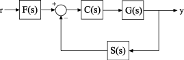
Suppose that the plant response is G(s)=1/(s+1)2, and that the model of the sensor dynamics is S(s)=5/(s+4). The controller C is a tunable PID controller, and the prefilter F=a/(s+a) is a low-pass filter with one tunable parameter, a.

Create models representing the plant and sensor dynamics. Because the plant and sensor dynamics are fixed, represent them using numeric LTI models.

G = zpk([],[-1,-1],1);
S = tf(5,[1 4]);

To model the tunable components, use Control Design Blocks. Create a tunable representation of the controller C.

C = tunablePID('C','PID');

C is a tunablePID object, which is a Control Design Block with a predefined proportional-integral-derivative (PID) structure.

Create a model of the filter F=a/(s+a) with one tunable parameter.

a = realp('a',10); 
F = tf(a,[1 a]);

a is a realp (real tunable parameter) object with initial value 10. Using a as a coefficient in tf creates the tunable genss model object F.

Interconnect the models to construct a model of the complete closed-loop response from r to y.

T = feedback(G*C,S)*F
Generalized continuous-time state-space model with 1 outputs, 1 inputs, 5 states, and the following blocks:
  C: Tunable PID controller, 1 occurrences.
  a: Scalar parameter, 2 occurrences.

Type "ss(T)" to see the current value and "T.Blocks" to interact with the blocks.

T is a genss model object. In contrast to an aggregate model formed by connecting only numeric LTI models, T keeps track of the tunable elements of the control system. The tunable elements are stored in the Blocks property of the genss model object. Examine the tunable elements of T.

T.Blocks
ans = struct with fields:
    C: [1x1 tunablePID]
    a: [1x1 realp]

When you create a genss model of a control system that has tunable components, you can use tuning commands such as systune to tune the free parameters to meet design requirements you specify.

Create a genss model with labeled state names. To do so, label the states of the component LTI models before connecting them. For instance, connect a two-state fixed-coefficient plant model and a one-state tunable controller.

A = [-1 -1; 1 0];
B = [1; 0];
C = [0 1];
D = 0;
G = ss(A,B,C,D);
G.StateName = {'Pstate1','Pstate2'};

C = tunableSS('C',1,1,1);

L = G*C;

The genss model L preserves the state names of the components that created it. Because you did not assign state names to the tunable component C, the software automatically does so. Examine the state names of L to confirm them.

L.StateName
ans = 3x1 cell
    {'Pstate1'}
    {'Pstate2'}
    {'C.x1'   }

The automatic assignment of state names to control design blocks allows you to trace which states in the generalized model are contributed by tunable components.

State names are also preserved when you convert a genss model to a fixed-coefficient state-space model. To confirm, convert L to ss form.

Lfixed = ss(L);
Lfixed.StateName
ans = 3x1 cell
    {'Pstate1'}
    {'Pstate2'}
    {'C.x1'   }

State unit labels, stored in the StateUnit property of the genss model, behave similarly.

Create a generalized model with a tunable parameter, and examine the dependence of the A matrix on that parameter. To do so, examine the A property of the generalized model.

G = tf(1,[1 10]);
k = realp('k',1);
F = tf(k,[1 k]);
L1 = G*F;
L1.A
Generalized matrix with 2 rows, 2 columns, and the following blocks:
  k: Scalar parameter, 2 occurrences.

Type "double(ans)" to see the current value and "ans.Blocks" to interact with the blocks.

The A property is a generalized matrix that preserves the dependence on the real tunable parameter k. The state-space matrix properties A, B, C, and D only preserve dependencies on static parameters. When the genss model has dynamic control design blocks, these are set to their current value for evaluating the state-space matrix properties. For example, examine the A matrix property of a genss model with a tunable PI block.

C = tunablePID('C','PI');
L2 = G*C;
L2.A
ans = 2×2

  -10.0000    0.0010
         0         0

Here, the A matrix is stored as a double matrix, whose value is the A matrix of the current value of L2.

L2cur = ss(L2);
L2cur.A
ans = 2×2

  -10.0000    0.0010
         0         0

Additionally, extracting state-space matrices using ssdata sets all control design blocks to their current or nominal values, including static blocks. Thus, the following operations all return the current value of the A matrix of L1.

[A,B,C,D] = ssdata(L1);
A
A = 2×2

   -10     1
     0    -1

double(L1.A)
ans = 2×2

   -10     1
     0    -1

L1cur = ss(L1);
L1cur.A
ans = 2×2

   -10     1
     0    -1

Tips

  • You can manipulate genss models as ordinary ss models. Analysis commands such as bode and step evaluate the model by replacing each tunable parameter with its current value.

Version History

Introduced in R2011a