coverage

Display or compute coverage map

Since R2019b

Syntax

coverage(txs)

coverage(txs,propmodel)

coverage(txs,rx)

coverage(txs,rx,propmodel)

coverage(___,Name,Value,___)

pd = coverage(txs,___)

Description

coverage(txs) displays the coverage map for the specified transmitter site in the current Site Viewer. Each colored contour of the map defines an area where the corresponding signal strength is transmitted to the mobile receiver.

Note

This function only supports antenna sites with CoordinateSystem property set to "geographic".

coverage(txs,propmodel) displays the coverage map based on the specified propagation model. The default propagation model is "longley-rice" when terrain is in use and "freespace" when terrain is not used.

coverage(txs,rx) displays the coverage map based on the receiver site properties.

coverage(txs,rx,propmodel) displays the coverage map based on the receiver site properties and specified propagation model.

coverage(___,Name,Value,___) displays the coverage map using additional options specified by the Name,Value pairs.

pd = coverage(txs,___) returns computed coverage data in the propagation data object, pd. No plot is displayed and any graphical only name-value pairs are ignored.

Examples

Coverage Map of Transmitter

Create a transmitter site at MathWorks headquarters.

tx = txsite('Name','MathWorks', ...
        'Latitude', 42.3001, ...
        'Longitude', -71.3503);

Show the coverage map.

coverage(tx)

Coverage Map Using Transmitter and Receiver

Create a transmitter site at MathWorks headquarters.

tx = txsite('Name','MathWorks', ...
        'Latitude', 42.3001, ...
        'Longitude', -71.3503);

Create a receiver site at Fenway Park with an antenna height of 1.2 m and system loss of 10 dB.

rx = rxsite('Name','Fenway Park', ...
       'Latitude',42.3467, ...
       'Longitude',-71.0972,'AntennaHeight',1.2,'SystemLoss',10);

Calculate the coverage area of the transmitter using a close-in propagation model.

coverage(tx,rx,'PropagationModel','closein')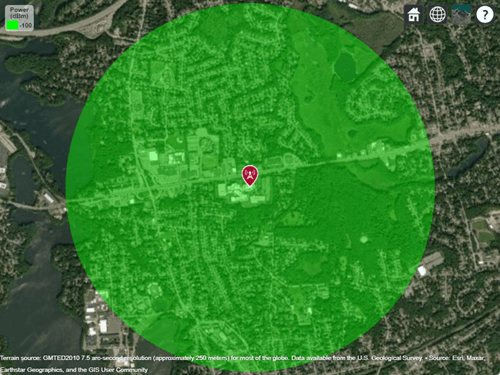

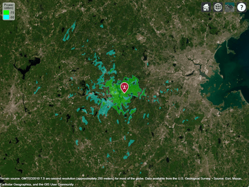
Coverage Map for Strong and Weak Signals

Define strong and weak signal strengths with corresponding colors.

strongSignal = -75;
strongSignalColor = "green";
weakSignal = -90;
weakSignalColor = "cyan";

Create a transmitter site and display the coverage map.

tx = txsite('Name','MathWorks', ...
    'Latitude',42.3001, ...
    'Longitude',-71.3503);
coverage(tx, ...
    'SignalStrengths',[strongSignal,weakSignal], ...
    'Colors', [strongSignalColor,weakSignalColor])

Combined Coverage Map of Multiple Transmitters

Define the names and the locations of sites around Boston.

names = ["Fenway Park","Faneuil Hall","Bunker Hill Monument"];
lats = [42.3467,42.3598,42.3763];
lons = [-71.0972,-71.0545,-71.0611];

Create the transmitter site array.

txs = txsite('Name', names,...
       'Latitude',lats,...
       'Longitude',lons, ...
       'TransmitterFrequency',2.5e9);

Display the combined coverage map for multiple signal strengths, using close-in propagation model.

coverage(txs,'close-in','SignalStrengths',-100:5:-60)

Coverage Map Using Longley-Rice and Ray Tracing Method

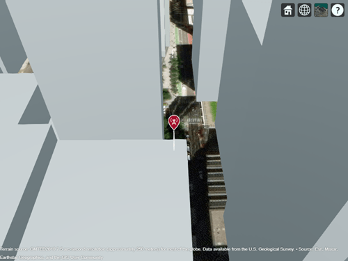
Launch Site Viewer using buildings in Chicago. For more information about the osm file, see [1].

viewer = siteviewer("Buildings","chicago.osm");

Create a transmitter site on a building.

tx = txsite("Latitude",41.8800, ...
   "Longitude",-87.6295, ...
   "TransmitterFrequency",2.5e9);
show(tx)

Coverage Map Using Longley-Rice Propagation Model

Create a coverage map of the city using the Longley-Rice propagation model.

coverage(tx,"SignalStrengths",-100:-5,"MaxRange",250,"Resolution",1)

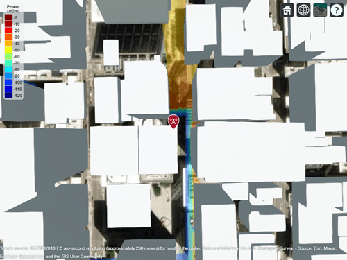
Longley-Rice models over-the-rooftops propagation along vertical slices and obstructions tend to dominate the coverage region.

Coverage Map Using Ray Tracing Propagation Model and Image Method

Create a ray tracing propagation model, which MATLAB® represents using a RayTracing object. Configure the model to use the image method and to find propagation paths with up to 1 surface reflection.

pmImage = propagationModel("raytracing","Method","image", ...
    "MaxNumReflections",1);

Create a coverage map of the city using the transmitter site and the ray tracing propagation model.

coverage(tx,pmImage,"SignalStrengths",-100:-5, ...
    "MaxRange",250,"Resolution",2)

This coverage map shows new regions that are in service due to reflected propagation paths.

Coverage Map Using Ray Tracing Propagation Model and SBR Method

Create another ray tracing propagation model. This time, configure the model to use the shooting and bouncing rays (SBR) method and to find propagation paths with up to 2 surface reflections. The SBR method is generally faster than the image method.

pmSBR = propagationModel("raytracing","Method","sbr", ...
    "MaxNumReflections",2);

Create an updated coverage map of the city.

coverage(tx,pmSBR,"SignalStrengths",-100:-5, ...
    "MaxRange",250,"Resolution",2)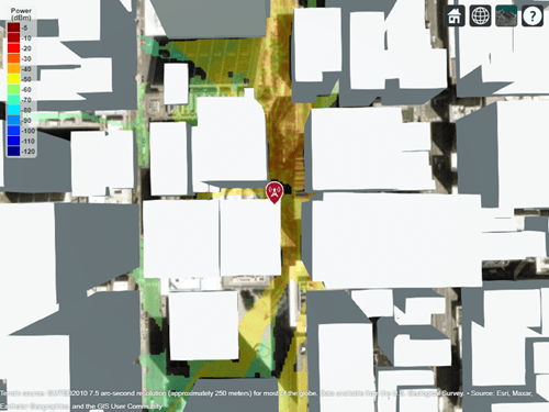

This coverage map shows new regions that are in service due to the additional reflected propagation paths.

Appendix

[1] The osm file is downloaded from https://www.openstreetmap.org, which provides access to crowd-sourced map data all over the world. The data is licensed under the Open Data Commons Open Database License (ODbL), https://opendatacommons.org/licenses/odbl/.

Input Arguments

txs — Transmitter sites

txsite object | array of txsite objects

Transmitter site, specified as a txsite object. Use array inputs to specify multiple sites.

This function only supports plotting antenna sites when CoordinateSystem property is set to "geographic".

rx — Receiver site

rxsite object

Receiver site, specified as a rxsite object.

This function only supports plotting antenna sites when CoordinateSystem property is set to "geographic".

propmodel — Propagation model to use for path loss calculations

"longley-rice" (default) | "freespace" | "close-in" | "rain" | "gas" | "fog" | "raytracing" | propagation model created using propagationModel

Propagation model to use for the path loss calculations, specified as one of these options:

• "freespace" — Free space propagation model

• "rain" — Rain propagation model

• "gas" — Gas propagation model

• "fog" — Fog propagation model

• "close-in" — Close-in propagation model

• "longley-rice" — Longley-Rice propagation model

• "tirem" — TIREM™ propagation model

• "raytracing" — Ray tracing propagation model that uses the shooting and bouncing rays (SBR) method. When you specify a ray tracing model as input, the function incorporates multipath interference by using a phasor sum.

• A propagation model created using the propagationModel function. For example, you can create a ray tracing propagation model that uses the image method by specifying propagationModel("raytracing","Method","image").

The default value depends on the coordinate system used by the input sites.

Coordinate System	Default propagation model value
"geographic"	"longley-rice" when you use a terrain. "freespace" when you do not use a terrain.
"cartesian"	"freespace" when Map is set to none. "raytracing" when Map is set to the name of an STL file or a triangulation object. The default ray tracing model uses the shooting and bouncing rays (SBR) method.

Terrain propagation models, including "longley-rice" and "tirem", are only supported for sites with a CoordinateSystem value of "geographic".

You can also specify the propagation model by using the PropagationModel name-value pair argument.

Name-Value Arguments

Specify optional pairs of arguments as Name1=Value1,...,NameN=ValueN, where Name is the argument name and Value is the corresponding value. Name-value arguments must appear after other arguments, but the order of the pairs does not matter.

Before R2021a, use commas to separate each name and value, and enclose Name in quotes.

Example: "Type","power"

Type — Type of signal strength to compute

"power" (default) | "efield"

Type of signal strength to compute, specified as one of these options:

• "power" — The signal strengths in SignalStrengths is in power units (dBm) of the signal at the mobile receiver input.

• "efield"— The signal strength in SignalStrengths is in electric field strength units (dBμV/m) of signal wave incident on the antenna.

Data Types: char | string

SignalStrengths — Signal strengths to display on coverage map

numeric vector

Signal strengths to display on coverage map, specified as a numeric vector.

Each strength uses different colored filled contour on the map. The default value is -100 dBm if Type is "power" and 40 dBμV/m if Type is "efield".

Data Types: double

PropagationModel — Propagation model to use for path loss calculations

"freespace" | "close-in" | "rain" | "gas" | "fog" | "longley-rice" | "raytracing" | propagation model created using propagationModel

Propagation model to use for the path loss calculations, specified as one of these options:

• "freespace" — Free space propagation model

• "rain" — Rain propagation model

• "gas" — Gas propagation model

• "fog" — Fog propagation model

• "close-in" — Close-in propagation model

• "longley-rice" — Longley-Rice propagation model

• "tirem" — TIREM propagation model

• "raytracing" — Ray tracing propagation model that uses the shooting and bouncing rays (SBR) method. When you specify a ray tracing model as input, the function incorporates multipath interference by using a phasor sum.

• A propagation model created using the propagationModel function. For example, you can create a ray tracing propagation model that uses the image method by specifying propagationModel("raytracing","Method","image").

The default value depends on the coordinate system used by the input sites.

Coordinate System	Default propagation model value
"geographic"	"longley-rice" when you use a terrain. "freespace" when you do not use a terrain.
"cartesian"	"freespace" when Map is set to none. "raytracing" when Map is set to the name of an STL file or a triangulation object. The default ray tracing model uses the shooting and bouncing rays (SBR) method.

Terrain propagation models, including "longley-rice" and "tirem", are only supported for sites with a CoordinateSystem value of "geographic".

Data Types: char | string

MaxRange — Maximum range of coverage map from each transmitter site

numeric scalar

Maximum range of coverage map from each transmitter site, specified as a positive numeric scalar in meters representing great circle distance. MaxRange defines the region of interest on the map to plot. The default value is automatically computed based on the type of propagation model.

Type of Propagation Model	MaxRange
Atmospheric or empirical	Range of minimum value in SignalStrengths.
Terrain	30 km or distance to the furthest building.
Ray tracing	500 m

For more information about the types of propagation models, see Choose a Propagation Model.

Data Types: double

Resolution — Resolution of coverage map

"auto" (default) | numeric scalar

Resolution of coverage map, specified as "auto" or a numeric scalar in meters.

The resolution of "auto" computes the maximum value scaled to MaxRange. Decreasing the resolution increases the quality of the coverage map and the time required to create it.

Data Types: char | string | double

ReceiverGain — Mobile receiver gain

2.1 (default) | numeric scalar

Mobile receiver gain, specified as a numeric scalar in dB. The receiver gain value includes the mobile receiver antenna gain and system loss.

The receiver gain computes received signal strength when Type is "power".

If receiver site argument rx is passed to coverage, the default value is the maximum gain of the receiver antenna with the system loss subtracted. Otherwise the default value is 2.1.

Data Types: char | string | double

ReceiverAntennaHeight — Mobile receiver antenna height above ground elevation

1 (default) | numeric scalar

Mobile receiver antenna height above ground elevation, specified as a numeric scalar in meters.

If receiver site argument rx is passed to coverage, the default value is the AntennaHeight of the receiver. Otherwise the default value is 1.

Data Types: double

Colors — Colors of filled contours on coverage map

M-by-3 array of RGB triplets | array of strings | cell array of character vectors

Colors of filled contours on coverage map, specified as one of these options:

• An M-by-3 array of RGB triplets whose elements specify the intensities of the red, green, and blue components of the color. The intensities must be in the range [0,1]; for example, [0.4 0.6 0.7].

• An array of strings such as ["red" "green" "blue"] or ["r" "g" "b"].

• A cell array of character vectors such as {'red','green','blue'} or {'r','g','b'}.

Colors are assigned element-wise to SignalStrengths values for coloring the corresponding filled contours.

Colors cannot be used with ColorLimits or ColorMap.

This table contains the color names and equivalent RGB triplets for some common colors.

Color Name	Short Name	RGB Triplet	Appearance
"red"	"r"	[1 0 0]
"green"	"g"	[0 1 0]
"blue"	"b"	[0 0 1]
"cyan"	"c"	[0 1 1]
"magenta"	"m"	[1 0 1]
"yellow"	"y"	[1 1 0]
"black"	"k"	[0 0 0]
"white"	"w"	[1 1 1]

Data Types: char | string | double

ColorLimits — Color limits for colormap

two-element vector

Color limits for colormap, specified as a two-element vector of type [min max].

The color limits indicate the signal level values that map to the first and last colors on the colormap.

The default value is [-120 -5] if the Type is "power" and [20 135] if Type is "efield".

ColorLimits cannot be used with Colors.

Data Types: double

ColorMap — Colormap filled contours for coverage map

"jet" (default) | predefined color map | M-by-3 array of RGB triplets

Colormap filled contours on coverage map, specified as a predefined colormap or M-by-3 array of RGB triplets, where M defines individual colors.

ColorMap cannot be used with Colors.

Data Types: char | string | double

ShowLegend — Show signal strength color legend on map

true (default) | false

Show signal strength color legend on map, specified as true or false.

Data Types: logical

Transparency — Transparency of coverage map

0.4 (default) | numeric scalar

Transparency of coverage map, specified as a numeric scalar in the range 0 to 1. 0 is transparent and 1 is opaque.

Data Types: double

Map — Map for visualization of surface data

siteviewer object

Map for visualization of surface data, specified as a siteviewer object.¹

Data Types: char | string

Output Arguments

pd — Coverage data

propagationData object

Coverage data, returned as a propagationData object consisting of Latitude and Longitude, and a signal strength variable corresponding to the plot type. Name of the propagationData is "Coverage Data".

Limitations

When you specify a RayTracing object as input to the coverage function, the value of the MaxNumDiffractions property must be 0 or 1.

Version History

Introduced in R2019b

R2023a: Ray tracing models discard paths based on path loss

Ray tracing propagation models discard propagation paths based on path loss thresholds. By default, when you specify the propmodel input argument as "raytracing" or a RayTracing object, the propagation model discards paths that are more than 40 dB weaker than the strongest path.

As a result, the coverage function can return different values in R2023a compared to previous releases. To avoid discarding paths based on relative path loss thresholds, create a RayTracing object (by using the propagationModel function) and set its MaxRelativePathLoss property to Inf. Then, use the object as input to the coverage function.

R2022b: Ray tracing functions consider multipath interference

When calculating received power using ray tracing models, the coverage function now incorporates multipath interference by using a phasor sum. In previous releases, the function used a power sum. As a result, the calculations in R2022b are more accurate than in previous releases.

R2021b: "raytracing" propagation models use SBR method

Starting in R2021b, when you use the coverage function and specify the propmodel argument or PropagationModel name-value argument as "raytracing", the function uses the shooting and bouncing rays (SBR) method and calculates up to two reflections. In previous releases, the coverage function uses the image method and calculates up to one reflection.

To display or compute coverage maps using the image method instead, create a propagation model by using the propagationModel function. Then, use the coverage function with the propagation model as input. This example shows how to update your code.

pm = propagationModel("raytracing","Method","image");
coverage(txs,pm)

For information about the SBR and image methods, see Choose a Propagation Model.

Starting in R2021b, all RF Propagation functions use the SBR method by default and calculate up to two reflections. For more information, see Default modeling method is shooting and bouncing rays method.

References

[1] International Telecommunications Union Radiocommunication Sector. Effects of Building Materials and Structures on Radiowave Propagation Above About 100MHz. Recommendation P.2040. ITU-R, approved August 23, 2023. https://www.itu.int/rec/R-REC-P.2040/en.
[2] International Telecommunications Union Radiocommunication Sector. Electrical Characteristics of the Surface of the Earth. Recommendation P.527. ITU-R, approved September 27, 2021. https://www.itu.int/rec/R-REC-P.527/en.
[3] Mohr, Peter J., Eite Tiesinga, David B. Newell, and Barry N. Taylor. “Codata Internationally Recommended 2022 Values of the Fundamental Physical Constants.” NIST, May 8, 2024. https://www.nist.gov/publications/codata-internationally-recommended-2022-values-fundamental-physical-constants.
[4] "IEEE Standard Definitions of Terms for Antennas." IEEE Std 145-2013 (Revision of IEEE Std 145-1993), March 2014, 1–50. https://doi.org/10.1109/IEEESTD.2014.6758443.
Extended Capabilities
The coverage function supports ray
tracing analysis on a GPU with these usage notes and limitations:
The function runs on the GPU when you specify a
RayTracingpropagation model object as input and theUseGPUproperty of the object is"on"or"auto".For information about when the GPU can accelerate ray tracing analysis, see the
UseGPUproperty of theRayTracingobject.In some cases, the GPU and local CPU results can differ due to small differences in algorithms and hardware implementations.
For an example that shows how to perform ray tracing analysis on a GPU, see Accelerate Ray Tracing Analysis Using GPU.