conformalArray
Create conformal array
Description
The conformalArray object creates a conformal array of the
specified antenna, array, or shape. You can also specify an array of any arbitrary
geometry, such as a circular array, a nonplanar array, an array with nonuniform
geometry, or a conformal array of arrays.
Conformal arrays are used in:
Direction-finding systems that use circular arrays or stacked circular arrays.
Aircraft systems due to surface irregularities or mechanical stress.
Creation
Description
c = conformalArraydipole
object resonating around 700 MHz and a center-fed
bowtieTriangular object resonating around 403 MHz when
isolated. The antennas are spaced 0.15m apart from each other along the
positive z-axis.
c = conformalArray(PropertyName=Value)PropertyName is the
property name and Value is the corresponding value. You
can specify several name-value arguments in any order as
PropertyName1=Value1,...,PropertyNameN=ValueN.
Properties that you do not specify, retain default values.
For example, c = conformalArray(Element={dipole
monopole},ElementPosition=[0,0,0.1; 0,0,0.2]) creates a
conformal array of a dipole and a monopole antenna whose feeds are at a
distance of 0.1 m and 0.2 m from the origin along the positive
z-axis.
Properties
Object Functions
arrayFactor | Array factor in dB |
axialRatio | Calculate and plot axial ratio of antenna or array |
beamwidth | Beamwidth of antenna |
charge | Charge distribution on antenna or array surface |
correlation | Correlation coefficient between two antennas in array |
current | Current distribution on antenna or array surface |
design | Create antenna, array, or AI-based antenna resonating at specified frequency |
doa | Direction of arrival of signal |
efficiency | Calculate and plot radiation efficiency of antenna or array |
EHfields | Electric and magnetic fields of antennas or embedded electric and magnetic fields of antenna element in arrays |
feedCurrent | Calculate current at feed for antenna or array |
impedance | Calculate and plot input impedance of antenna or scan impedance of array |
info | Display information about antenna, array, or platform |
layout | Display array or PCB stack layout |
memoryEstimate | Estimate memory required to solve antenna or array mesh |
mesh | Generate and view mesh for antennas, arrays, and custom shapes |
meshconfig | Change meshing mode of antenna, array, custom antenna, custom array, or custom geometry |
msiwrite | Write antenna or array analysis data to MSI planet file |
optimize | Optimize antenna and array catalog elements using SADEA or TR-SADEA algorithm |
pattern | Plot radiation pattern of antenna, array, or embedded element of array |
patternAzimuth | Azimuth plane radiation pattern of antenna or array |
patternElevation | Elevation plane radiation pattern of antenna or array |
patternMultiply | Radiation pattern of array using pattern multiplication |
peakRadiation | Calculate and mark maximum radiation points of antenna or array on radiation pattern |
phaseShift | Calculate phase shift values for arrays or multi-feed PCB stack |
rcs | Calculate and plot monostatic and bistatic radar cross section (RCS) of platform, antenna, or array |
returnLoss | Calculate and plot return loss of antenna or scan return loss of array |
show | Display antenna, array, AI-based antenna, platform, or shape |
sparameters | Calculate S-parameters for antenna or array |
stlwrite | Write mesh information to STL file |
vswr | Calculate and plot voltage standing wave ratio (VSWR) of antenna or array element |
Examples
Create a default conformal array.
c = conformalArray
c =
  conformalArray with properties:

            Element: {[1×1 dipole]  [1×1 bowtieTriangular]}
    ElementPosition: [2×3 double]
          Reference: 'feed'
     AmplitudeTaper: 1
         PhaseShift: 0
               Tilt: 0
           TiltAxis: [1 0 0]
show(c)
This example shows how to create a conformal array consisting of bowtieRounded, bowtieTriangular, dipoleBlade, and loopCircular antennas operating at 1 GHz. The same workflow using Antenna Array Designer app is also shown in a complementary video.
Video Walkthrough
For a walkthrough of the example, play the video.
Design and Analysis Workflow
Define the analysis frequency range.
f = 900e6:10e6:1.1e9;
Design and orient the rounded bowtie, triangular bowtie, blade dipole, and circular loop antennas.
% Rounded bowtie antenna
br = design(bowtieRounded,f(11));
br.Tilt = 90;
br.TiltAxis = [0 1 0];

% Triangular bowtie antenna
bt = design(bowtieTriangular,f(11));
bt.Tilt = 90;
bt.TiltAxis = [0 1 0];

% Blade dipole antenna
db = design(dipoleBlade,f(11));
db.Tilt = 90;
db.TiltAxis = [0 1 0];

% Circular loop antenna
lc = design(loopCircular,f(11));
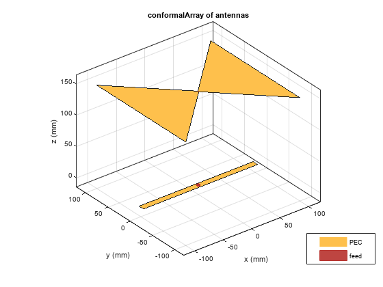
Create a conformal array.
c = conformalArray(Element={br bt db lc},...
    ElementPosition=[0.2189 0.2318 0; 0 0 0.2; -0.1 0.4 0; 0.4 0.6 0],Reference="origin")
c =
conformalArray with properties:
Element: {[1×1 bowtieRounded] [1×1 bowtieTriangular] [1×1 dipoleBlade] [1×1 loopCircular]}
ElementPosition: [4×3 double]
Reference: "origin"
AmplitudeTaper: 1
PhaseShift: 0
Tilt: 0
TiltAxis: [1 0 0]
Visualize the conformal array.
show(c)
Plot the S-parameters of this array in the 900 MHz to 1.1 GHz range.
s = sparameters(c,f);
figure
rfplot(s,{[1,1];[2,2];[3,3];[4,4]});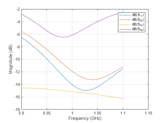
Plot the radiation pattern of this array at 1 GHz.
pattern(c,f(11))
Define the radius and the number of elements for the array.
r = 2;
N = 12;
Create an array of 12 dipoles.
elem = repmat(dipole(Length=1.5),1,N);
Define the x,y,z values for the element positions in the array.
del_th = 360/N;
th = del_th:del_th:360;
x = r.*cosd(th);
y = r.*sind(th);
z = ones(1,N);
pos = [x;y;z];
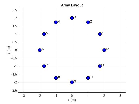
Create a circular array using the defined dipoles and then visualize it. Display the layout of the array.
c = conformalArray(Element=elem,ElementPosition=pos');
show(c)
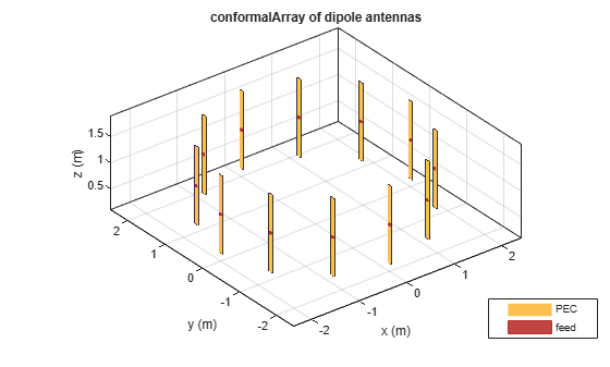
figure
layout(c)
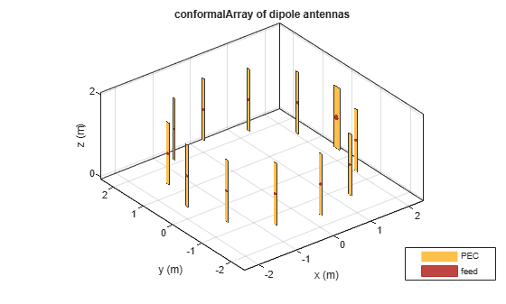
Change the width of the fourth and the twelfth element of the circular array. Visualize the new arrangement.
c.Element(4).Width = 0.05;
c.Element(12).Width = 0.2;
figure
show(c)
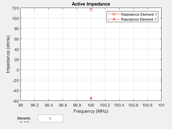
Calculate and plot the impedance of the circular array at 100 MHz. The plot shows the impedance of the first element in the array.
figure
impedance(c,100e6)
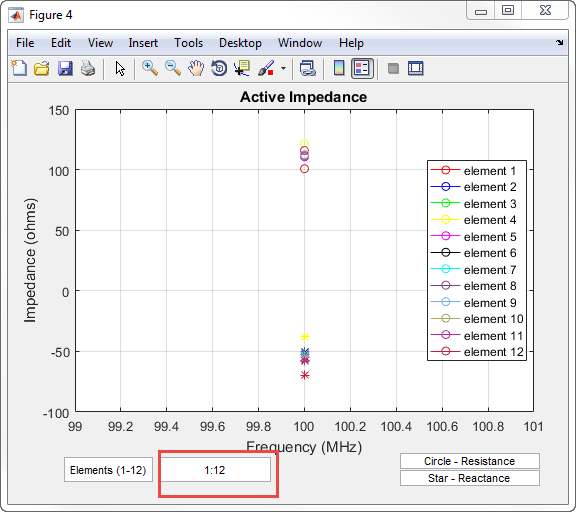
To view the impedance of all the elements in the array change the value from 1 to 1:12 as shown in the figure.
Define three circular loop antennas of radii 0.6366 m (default), 0.85 m, and 1 m, respectively.
l1 = loopCircular;
l2 = loopCircular(Radius=0.85);
l3 = loopCircular(Radius=1);
Create a concentric array that uses the origin of circular loop antennas as its position reference.
c = conformalArray(Element={l1 l2 l3},ElementPosition=[0 0 0; 0 0 0;...
     0 0 0],Reference="origin");
show(c)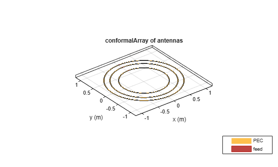
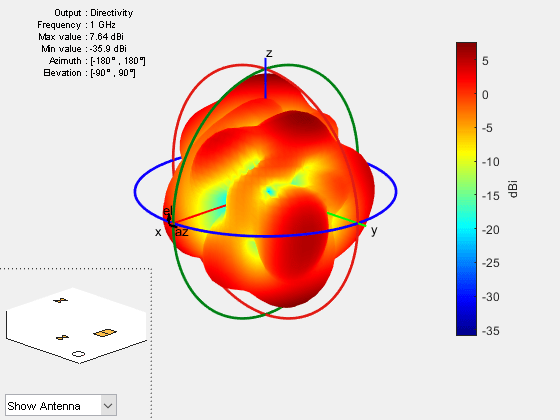
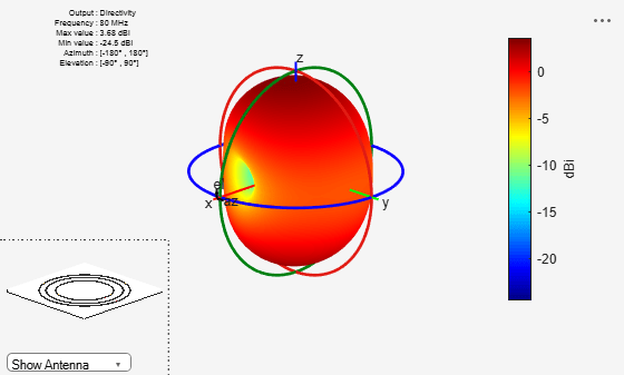
Visualize the radiation pattern of the array at 80 MHz.
pattern(c,80e6)
Create a dipole antenna to use in the reflector and the conformal array.
d = dipole(Length=0.13,Width=5e-3,Tilt=90,TiltAxis='Y');Create an infinite groundplane reflector antenna using the dipole as exciter.
rf = reflector(Exciter=d,Spacing=0.15/2,GroundPlaneLength=inf);
Create a conformal array using 36 dipole antennas and one infinite groundplane reflector antenna. View the array.
x = linspace(-0.4,0.4,6);
y = linspace(-0.4,0.4,6);
[X,Y] = meshgrid(x,y);
pos = [X(:) Y(:) 0.15*ones(numel(X),1)];
for i = 1:36
    element{i} = d;
end
element{37} = rf;
lwa = conformalArray(Element=element,ElementPosition=[pos; 0 0 0.15/2]);
show(lwa)
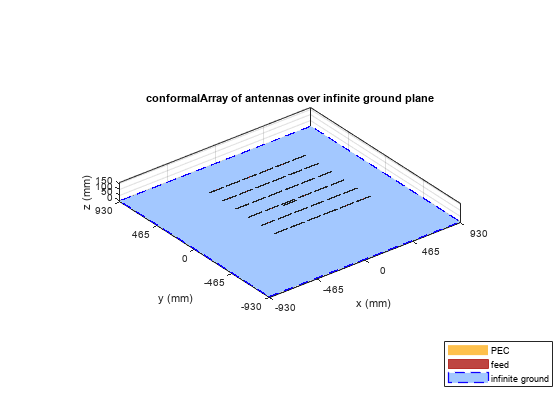
Drive only the reflector antenna with an amplitude of 1.
V = zeros(1,37);
V(end) = 1;
lwa.AmplitudeTaper = V;
Compute the radiation pattern of the conformal array.
figure
pattern(lwa,1e9,Type='efield')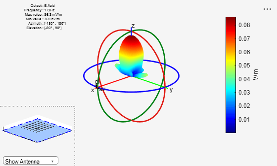
Create two patch microstrip antennas using dielectric substrate FR4. Tilt the second patch microstrip antenna by 180 degrees.
p1 = patchMicrostrip(Substrate=dielectric('FR4'));
p2 = patchMicrostrip(Substrate=dielectric('FR4'),Tilt=180);
Create and view a conformal array using the two patch microstrip antennas placed 11 cm apart.
c = conformalArray(ElementPosition=[0 0 0; 0 0 0.1100],Element={p1 p2});
show(c)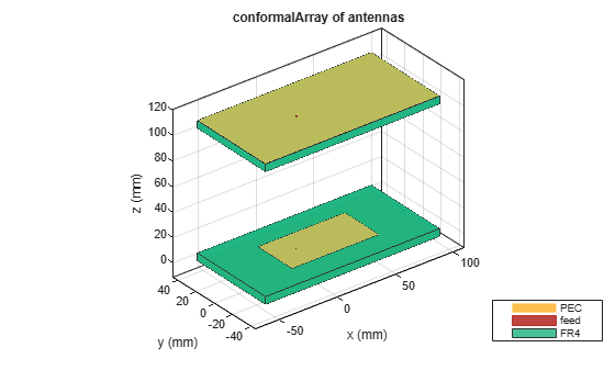
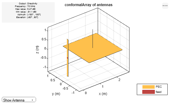
Create a conformal array using dipole and monopole antennas and display it.
c = conformalArray(Element={dipole monopole},...
    ElementPosition=[0 0 0; 1.5 0 0]);
show(c)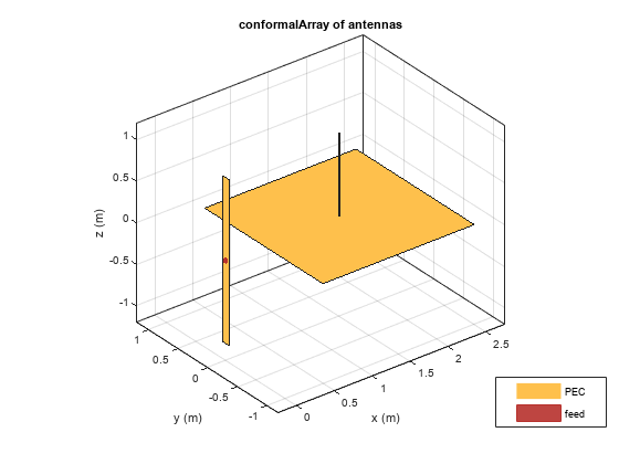
Plot the radiation pattern of the array at 70 MHz.
pattern(c,70e6)
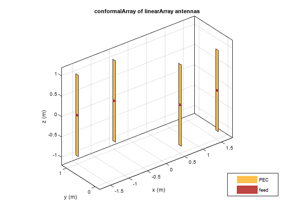
Create a subarray of linear arrays at different locations.
la = linearArray(ElementSpacing=1)
la =
  linearArray with properties:

           Element: [1×1 dipole]
       NumElements: 2
    ElementSpacing: 1
    AmplitudeTaper: 1
        PhaseShift: 0
              Tilt: 0
          TiltAxis: [1 0 0]
subArr = conformalArray(Element=[la la],ElementPosition=[1 0 0; -1 1 0])
subArr =
  conformalArray with properties:

            Element: [1×2 linearArray]
    ElementPosition: [2×3 double]
          Reference: 'feed'
     AmplitudeTaper: 1
         PhaseShift: 0
               Tilt: 0
           TiltAxis: [1 0 0]
show(subArr)
Create a linear array of dipoles with and element spacing of 1m.
la = linearArray(ElementSpacing=1);
Create a rectangular array of microstrip patch antennas.
ra = rectangularArray(Element=patchMicrostrip,RowSpacing=0.1,ColumnSpacing=0.1);
Create a subarray containing the above linear and rectangular arrays with changes in amplitude taper and phase shift values.
subArr = conformalArray(Element={la ra dipole},ElementPosition=[0 0 1.5; 0 0 0; 1 1 1],...
    AmplitudeTaper=[3 0.3 0.03],PhaseShift=[90 180 120]);
show(subArr)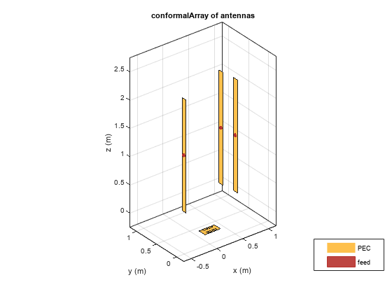
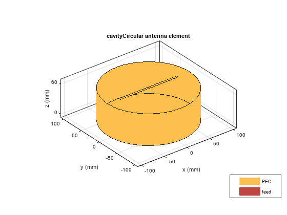
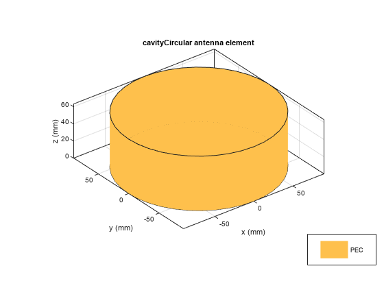
This example shows how to create a circular cavity structure as an element in a conformalArray and plot its surface current distribution.
Create Circular Cavity Antenna
Create a circular cavity antenna operating at 1 GHz using the design function and the cavityCircular element from the antenna catalog. Display the antenna.
f = 1e9;
lambda = 3e8/f;
ant = design(cavityCircular,f);
figure
show(ant)
Derive Backing Structure
Derive the circular cavity backing structure from the cavity antenna by specifying the 'Exciter' property as an empty array. Display the backing structure.
ant.Exciter = [];
figure
show(ant)
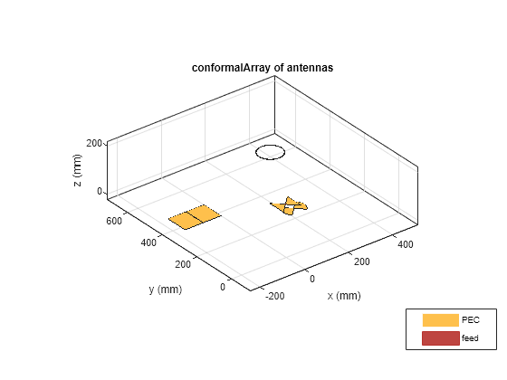
Create Conformal Array
Create and display a conformal array with circular cavity as one of its elements.
ca = conformalArray;
ca.Reference = "origin";
ca.ElementPosition = [0 0 0; 0 0 0.25; 0 0 0.5];
ca.Element = {ca.Element{1} ant ca.Element{2}};
figure
show(ca)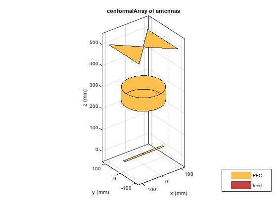
Plot Surface Current Distribution
Calculate the current at the feed location and plot the surface current distribution of the conformal array at 1 GHz.
If = feedCurrent(ca,f)
If = 1×2 complex

   0.0023 - 0.0005i   0.0029 + 0.0007i
figure
current(ca,f,Scale="log10")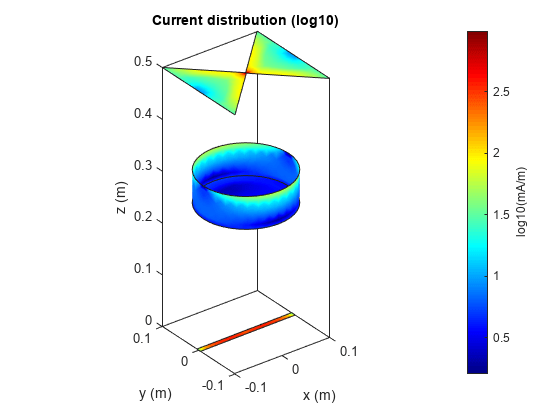
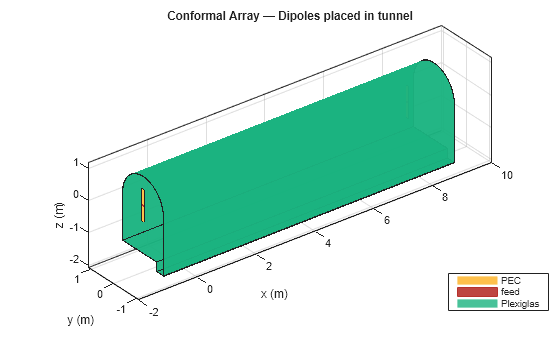
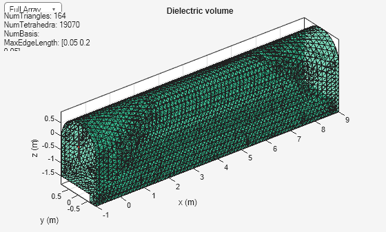
This example shows how to create a conformal array of antennas and a geometric structure. This example uses two dipole antennas and a Plexiglas tunnel for the demonstration. The dipole antennas are placed at the openings of the tunnel.
Define the dimensions in meters.
domeRadius = 1.8/2;
outlineWidth = 1.5;
cavityLength = 0.3;
cavityWidth = 0.3;
thickness = 0.01;
tunnelLength = 10;
Create two tunnel faces with slightly different dimensions. Then subtract smaller face from the larger to get an outline of the tunnel with specified thickness. Create shapes for tunnel dome, wall, and cavity. Add them together to get the overall shape.
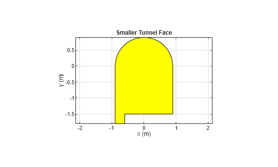
Create smaller tunnel face.
tunnelDome = shape.Circle(Radius=domeRadius);
tunnelWall = shape.Rectangle(Length=domeRadius*2,Width=outlineWidth);
[~] = translate(tunnelWall,[0 -tunnelWall.Width/2 0]);
tunnelCavity = shape.Rectangle(Length=cavityLength,Width=cavityWidth);
[~] = translate(tunnelCavity,[-tunnelWall.Length/2+tunnelCavity.Length/2 ...
    -tunnelWall.Width-tunnelCavity.Width/2 0 ]);
tunnelSmall = tunnelDome + tunnelWall + tunnelCavity;
figure
show(tunnelSmall)
title("Smaller Tunnel Face")
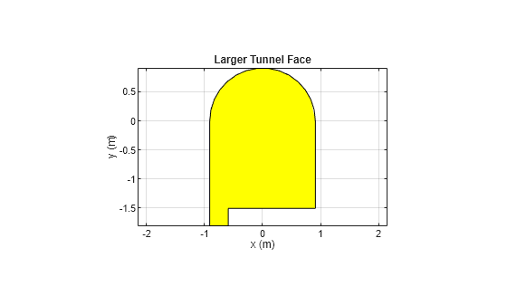
Create larger tunnel face.
tunnelDome = shape.Circle(Radius=domeRadius+thickness);
tunnelWall = shape.Rectangle(Length=domeRadius*2+thickness*2,Width=outlineWidth+thickness);
[~] = translate(tunnelWall,[0 -tunnelWall.Width/2 0]);
tunnelCavity = shape.Rectangle(Length=cavityLength+thickness*2,Width=cavityWidth);
[~] = translate(tunnelCavity,[-tunnelWall.Length/2+tunnelCavity.Length/2 ...
    -tunnelWall.Width-tunnelCavity.Width/2 0 ]);
tunnelLarge = tunnelDome + tunnelWall + tunnelCavity;
figure
show(tunnelLarge)
title("Larger Tunnel Face")
Subtract smaller face from larger to get an outline of the tunnel with 0.01 m thickness.
tunnelOutline = tunnelLarge - tunnelSmall;
show(tunnelOutline)
title("Outline of Tunnel with 0.01 m Thickness")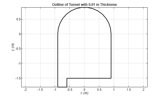
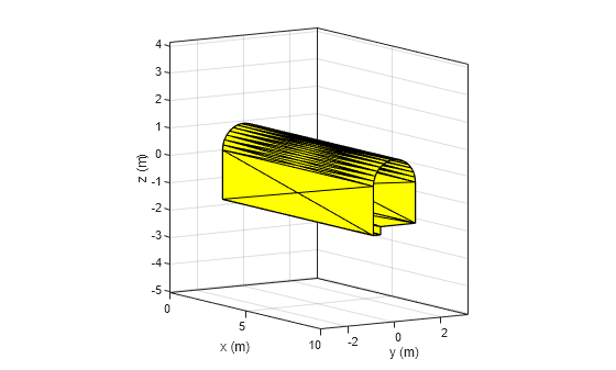
Linearly extrude the outline to generate a 10 m. long tunnel. Specify Plexiglas as the dielectric material of the tunnel using the Dielectric property. You can add any dielectric material from the dielectric catalog. To view a list of dielectric materials, run openDielectricCatalog on the command line.
tunnelOutline = removeSlivers(tunnelOutline,1e-12);
tunnel = extrudeLinear(tunnelOutline,tunnelLength,Caps=true)
tunnel =
  Custom3D with properties:

              Name: 'custom3D'
          Vertices: [80×3 double]
             Metal: 'PEC'
        Dielectric: 'Air'
    FrequencyModel: 'Constant'
             Color: 'y'
      Transparency: 1
         EdgeColor: 'k'
tunnel.Dielectric="Plexiglas";Orient the tunnel.
[~] = rotateY(tunnel,90);
rotateX(tunnel,90);
Create a conformal array with two dipoles and the tunnel as its elements.
c = conformalArray;
c.ElementPosition = [-1 0 0;-1 0 0;8 0 0];
c.Reference = "origin";
c.Element = {dipole(Length=1),tunnel,dipole(Length=1)};
figure
show(c)
title("Conformal Array — Dipoles placed in tunnel")
Mesh the conformal array. You can control the mesh of individual elements by specifying a vector of edge lengths.
mesh(c,MaxEdgeLength=[0.05 0.2 0.05]);
Define the inner and outer radius of the radome, and a scaling factor.
rad1 = 0.1;        % inner radius (m)
thick = 0.1*rad1;  % shell thickness (m)
fact = 2.2;        % scaling factor for the cutting box
Create a solid inner hemisphere with Plexiglass® material using a sphere and a box.
sph = shape.Sphere(Radius=rad1,Dielectric="Plexiglas");
box = shape.Box(Length=(rad1+thick)*fact,Width=(rad1+thick)*fact, ...
    Height=(rad1+thick)*fact,Dielectric="Plexiglas");
[~] = translate(box,[0 0 -box.Height/2]);
sph1 = subtract(sph,box,RetainShape=true);
vert1 = getShapeVertices(sph);
Create the outer hemisphere with the same dielectric material.
sph = shape.Sphere(Radius=rad1+thick,Dielectric="Plexiglas");
box = shape.Box(Length=(rad1+thick)*fact,Width=(rad1+thick)*fact, ...
    Height=(rad1+thick)*fact,Dielectric="Plexiglas");
[~] = translate(box,[0 0 -box.Height/2]);
sph2 = subtract(sph,box,RetainShape=true);
Add the inner and outer hemispheres. Mesh the resultant shape, and get the points and triangles of the mesh.
sph = sph1 + sph2;
[~] = mesh(sph,MaxEdgeLength=0.05);
[p,t] = exportMesh(sph);
Construct the final radome shape using triangulation and specify the dielectric material for the shape.
tr = triangulation(t(:,1:3),p);
sph = shape.Custom3D(tr);
sph.Dielectric="Plexiglas";
[~] = rotateY(sph,90);
[~] = rotateZ(sph,180);
Create a conformal array, and assign a horn antenna and the previously constructed radome as its elements.
conf = conformalArray;
conf.Element{1} = horn(Tilt=180,TiltAxis="Z");
conf.Element{2} = sph;
conf.ElementPosition(2,:)= [-0.2 0 0];
conf.Reference="origin";
View the conformal array.
figure
show(conf)
title("Conformal Array of Horn and Radome")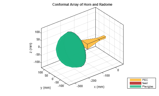
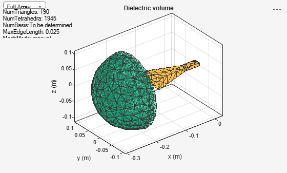
Mesh the conformal array with a 25 mm maximum edge length.
figure
mesh(conf,MaxEdgeLength=0.025);
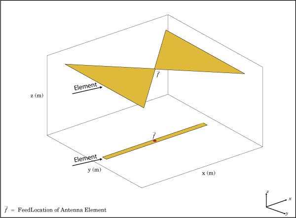
More About
Reference property of
conformalArray object defines the position reference of an
antenna element in 3–D space. You can position the antenna by specifying the
Reference property as "feed" or
"origin".
Choose the position reference as "feed" to move the antenna
element with respect to the feed point so that the new feed location is at the
specified coordinates. Following diagram shows a rectangular loop antenna and
reflector-backed antenna before and after relocation with respect to the feed
point:

Choose the position reference as "origin" to move the antenna
element so that new antenna origin is at the specified coordinates. Following
diagram shows a rectangular loop antenna and a reflector-backed antenna before and
after the relocation with respect to origin:

References
[1] Balanis, Constantine A. Antenna Theory: Analysis and Design. 3rd Ed. New York: John Wiley and Sons, 2005.