kmeans
k-means clustering
Syntax
Description
idx = kmeans(X,k)X
into k clusters, and returns an n-by-1 vector
(idx) containing cluster indices of each observation. Rows of
X correspond to points and columns correspond to variables.
By default, kmeans uses the squared Euclidean distance metric and the k-means++
algorithm for cluster center initialization.
idx = kmeans(X,k,Name,Value)Name,Value pair
arguments.
For example, specify the cosine distance, the number of times to repeat the clustering using new initial values, or to use parallel computing.
Examples
Cluster data using k-means clustering, then plot the cluster regions.
Load Fisher's iris data set. Use the petal lengths and widths as predictors.
load fisheriris
X = meas(:,3:4);

figure;
plot(X(:,1),X(:,2),'k*','MarkerSize',5);
title 'Fisher''s Iris Data';
xlabel 'Petal Lengths (cm)';
ylabel 'Petal Widths (cm)';
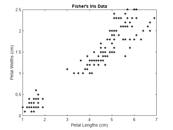
The larger cluster seems to be split into a lower variance region and a higher variance region. This might indicate that the larger cluster is two, overlapping clusters.
Cluster the data. Specify k = 3 clusters.
rng(1); % For reproducibility
[idx,C] = kmeans(X,3);
idx is a vector of predicted cluster indices corresponding to the observations in X. C is a 3-by-2 matrix containing the final centroid locations.
Use kmeans to compute the distance from each centroid to points on a grid. To do this, pass the centroids (C) and points on a grid to kmeans, and implement one iteration of the algorithm.
x1 = min(X(:,1)):0.01:max(X(:,1));
x2 = min(X(:,2)):0.01:max(X(:,2));
[x1G,x2G] = meshgrid(x1,x2);
XGrid = [x1G(:),x2G(:)]; % Defines a fine grid on the plot

idx2Region = kmeans(XGrid,3,'MaxIter',1,'Start',C);
Warning: Failed to converge in 1 iterations.
% Assigns each node in the grid to the closest centroidkmeans displays a warning stating that the algorithm did not converge, which you should expect since the software only implemented one iteration.
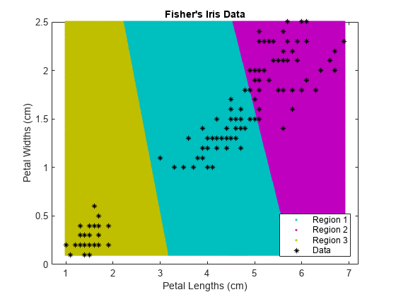
Plot the cluster regions.
figure;
gscatter(XGrid(:,1),XGrid(:,2),idx2Region,...
    [0,0.75,0.75;0.75,0,0.75;0.75,0.75,0],'..');
hold on;
plot(X(:,1),X(:,2),'k*','MarkerSize',5);
title 'Fisher''s Iris Data';
xlabel 'Petal Lengths (cm)';
ylabel 'Petal Widths (cm)';
legend('Region 1','Region 2','Region 3','Data','Location','SouthEast');
hold off;
Randomly generate the sample data.
rng default; % For reproducibility
X = [randn(100,2)*0.75+ones(100,2);
    randn(100,2)*0.5-ones(100,2)];

figure;
plot(X(:,1),X(:,2),'.');
title 'Randomly Generated Data';
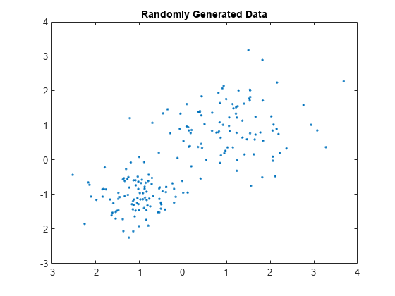
There appears to be two clusters in the data.
Partition the data into two clusters, and choose the best arrangement out of five initializations. Display the final output.
opts = statset('Display','final');
[idx,C] = kmeans(X,2,'Distance','cityblock',...
    'Replicates',5,'Options',opts);
Replicate 1, 3 iterations, total sum of distances = 0.9879171.79822.012450.8117850.42111.476630.935910.7658763.92211.979431.424072.662641.514380.8970231.211160.4900031.413872.344710.9618081.725542.639011.767771.526541.773070.474890.737131.323370.48160.7009451.910930.6884431.523612.030061.231352.433221.058281.000911.655061.244741.553550.3370910.4231971.308820.2056411.31780.8025581.036580.6277072.078681.509511.281030.1702011.127751.479361.012391.006141.158761.246460.3833821.036551.082730.6571421.011252.674342.354170.4094451.978721.251440.9742022.310791.506322.065221.276750.8709761.110391.63371.212310.4582970.5357611.03681.842510.5143450.5416491.19871.261181.256171.22131.371520.6112451.066731.0530.1301640.525781.910790.7818770.722291.450342.043190.5321252.058140.1718340.948870.720610.5322740.5367080.5896830.3956460.534580.5077240.3546260.728470.8935010.4712120.7593141.377580.7991450.6911630.2880741.129630.5508960.9993251.023740.7261060.2204910.9175090.4357990.5026970.2129291.156380.8346460.4969721.187010.5606991.044620.2570.4003661.135382.097341.43670.8821421.192170.5808720.2976160.401890.214231.58420.2424841.005980.4217950.1035350.8210810.1905330.4947271.102361.129220.3802381.103781.424281.211780.6076250.7203680.8542731.048020.5291860.6439461.002930.3392271.094660.1616450.3560030.8847070.6776620.9006650.332320.3368890.8842620.7647690.6776980.9044340.5589671.708050.8172460.3194670.8796910.9693671.099070.8290530.732971.020470.979410.2533961.089880.7817340.9302050.4414340.1001132.052320.634641.114861.52274.
Replicate 2, 5 iterations, total sum of distances = 0.9879171.79822.012450.8117850.42111.476630.935910.7658763.92211.979431.424072.662641.514380.8970231.211160.4900031.413872.344710.9618081.725542.639011.767771.526541.773070.474890.737131.323370.48160.7009451.910930.6884431.523612.030061.231352.433221.058281.000911.655061.244741.553550.3370910.4231971.308820.2056411.31780.8025581.036580.6277072.078681.509511.281030.1702011.127751.479361.012391.006141.158761.246460.3833821.036551.082730.6571421.011252.674342.354170.4094451.978721.251440.9742022.310791.506322.065221.276750.8709761.110391.63371.212310.4582970.5357611.03681.842510.5143450.5416491.19871.261181.256171.22131.371520.6112451.066731.0530.1301640.525781.910790.7818770.722291.450342.043190.5321252.058140.1718340.948870.720610.5322740.5367080.5896830.3956460.534580.5077240.3546260.728470.8935010.4712120.7593141.377580.7991450.6911630.2880741.129630.5508960.9993251.023740.7261060.2204910.9175090.4357990.5026970.2129291.156380.8346460.4969721.187010.5606991.044620.2570.4003661.135382.097341.43670.8821421.192170.5808720.2976160.401890.214231.58420.2424841.005980.4217950.1035350.8210810.1905330.4947271.102361.129220.3802381.103781.424281.211780.6076250.7203680.8542731.048020.5291860.6439461.002930.3392271.094660.1616450.3560030.8847070.6776620.9006650.332320.3368890.8842620.7647690.6776980.9044340.5589671.708050.8172460.3194670.8796910.9693671.099070.8290530.732971.020470.979410.2533961.089880.7817340.9302050.4414340.1001132.052320.634641.114861.52274.
Replicate 3, 3 iterations, total sum of distances = 0.9879171.79822.012450.8117850.42111.476630.935910.7658763.92211.979431.424072.662641.514380.8970231.211160.4900031.413872.344710.9618081.725542.639011.767771.526541.773070.474890.737131.323370.48160.7009451.910930.6884431.523612.030061.231352.433221.058281.000911.655061.244741.553550.3370910.4231971.308820.2056411.31780.8025581.036580.6277072.078681.509511.281030.1702011.127751.479361.012391.006141.158761.246460.3833821.036551.082730.6571421.011252.674342.354170.4094451.978721.251440.9742022.310791.506322.065221.276750.8709761.110391.63371.212310.4582970.5357611.03681.842510.5143450.5416491.19871.261181.256171.22131.371520.6112451.066731.0530.1301640.525781.910790.7818770.722291.450342.043190.5321252.058140.1718340.948870.720610.5322740.5367080.5896830.3956460.534580.5077240.3546260.728470.8935010.4712120.7593141.377580.7991450.6911630.2880741.129630.5508960.9993251.023740.7261060.2204910.9175090.4357990.5026970.2129291.156380.8346460.4969721.187010.5606991.044620.2570.4003661.135382.097341.43670.8821421.192170.5808720.2976160.401890.214231.58420.2424841.005980.4217950.1035350.8210810.1905330.4947271.102361.129220.3802381.103781.424281.211780.6076250.7203680.8542731.048020.5291860.6439461.002930.3392271.094660.1616450.3560030.8847070.6776620.9006650.332320.3368890.8842620.7647690.6776980.9044340.5589671.708050.8172460.3194670.8796910.9693671.099070.8290530.732971.020470.979410.2533961.089880.7817340.9302050.4414340.1001132.052320.634641.114861.52274.
Replicate 4, 3 iterations, total sum of distances = 0.9879171.79822.012450.8117850.42111.476630.935910.7658763.92211.979431.424072.662641.514380.8970231.211160.4900031.413872.344710.9618081.725542.639011.767771.526541.773070.474890.737131.323370.48160.7009451.910930.6884431.523612.030061.231352.433221.058281.000911.655061.244741.553550.3370910.4231971.308820.2056411.31780.8025581.036580.6277072.078681.509511.281030.1702011.127751.479361.012391.006141.158761.246460.3833821.036551.082730.6571421.011252.674342.354170.4094451.978721.251440.9742022.310791.506322.065221.276750.8709761.110391.63371.212310.4582970.5357611.03681.842510.5143450.5416491.19871.261181.256171.22131.371520.6112451.066731.0530.1301640.525781.910790.7818770.722291.450342.043190.5321252.058140.1718340.948870.720610.5322740.5367080.5896830.3956460.534580.5077240.3546260.728470.8935010.4712120.7593141.377580.7991450.6911630.2880741.129630.5508960.9993251.023740.7261060.2204910.9175090.4357990.5026970.2129291.156380.8346460.4969721.187010.5606991.044620.2570.4003661.135382.097341.43670.8821421.192170.5808720.2976160.401890.214231.58420.2424841.005980.4217950.1035350.8210810.1905330.4947271.102361.129220.3802381.103781.424281.211780.6076250.7203680.8542731.048020.5291860.6439461.002930.3392271.094660.1616450.3560030.8847070.6776620.9006650.332320.3368890.8842620.7647690.6776980.9044340.5589671.708050.8172460.3194670.8796910.9693671.099070.8290530.732971.020470.979410.2533961.089880.7817340.9302050.4414340.1001132.052320.634641.114861.52274.
Replicate 5, 2 iterations, total sum of distances = 0.9879171.79822.012450.8117850.42111.476630.935910.7658763.92211.979431.424072.662641.514380.8970231.211160.4900031.413872.344710.9618081.725542.639011.767771.526541.773070.474890.737131.323370.48160.7009451.910930.6884431.523612.030061.231352.433221.058281.000911.655061.244741.553550.3370910.4231971.308820.2056411.31780.8025581.036580.6277072.078681.509511.281030.1702011.127751.479361.012391.006141.158761.246460.3833821.036551.082730.6571421.011252.674342.354170.4094451.978721.251440.9742022.310791.506322.065221.276750.8709761.110391.63371.212310.4582970.5357611.03681.842510.5143450.5416491.19871.261181.256171.22131.371520.6112451.066731.0530.1301640.525781.910790.7818770.722291.450342.043190.5321252.058140.1718340.948870.720610.5322740.5367080.5896830.3956460.534580.5077240.3546260.728470.8935010.4712120.7593141.377580.7991450.6911630.2880741.129630.5508960.9993251.023740.7261060.2204910.9175090.4357990.5026970.2129291.156380.8346460.4969721.187010.5606991.044620.2570.4003661.135382.097341.43670.8821421.192170.5808720.2976160.401890.214231.58420.2424841.005980.4217950.1035350.8210810.1905330.4947271.102361.129220.3802381.103781.424281.211780.6076250.7203680.8542731.048020.5291860.6439461.002930.3392271.094660.1616450.3560030.8847070.6776620.9006650.332320.3368890.8842620.7647690.6776980.9044340.5589671.708050.8172460.3194670.8796910.9693671.099070.8290530.732971.020470.979410.2533961.089880.7817340.9302050.4414340.1001132.052320.634641.114861.52274.
Best total sum of distances = 201.533
By default, the software initializes the replicates separately using k-means++.
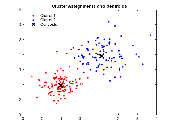
Plot the clusters and the cluster centroids.
figure;
plot(X(idx==1,1),X(idx==1,2),'r.','MarkerSize',12)
hold on
plot(X(idx==2,1),X(idx==2,2),'b.','MarkerSize',12)
plot(C(:,1),C(:,2),'kx',...
     'MarkerSize',15,'LineWidth',3)
legend('Cluster 1','Cluster 2','Centroids',...
       'Location','NW')
title 'Cluster Assignments and Centroids'
hold off
You can determine how well separated the clusters are by passing idx to silhouette.
Clustering large data sets might take time, particularly if you use online updates (set by default). If you have a Parallel Computing Toolbox™ license and you set the options for parallel computing, then kmeans runs each clustering task (or replicate) in parallel. And, if Replicates>1, then parallel computing decreases time to convergence.
Randomly generate a large data set from a Gaussian mixture model.
rng(1); % For reproducibility
Mu = ones(20,30).*(1:20)'; % Gaussian mixture mean
rn30 = randn(30,30);
Sigma = rn30'*rn30; % Symmetric and positive-definite covariance
Mdl = gmdistribution(Mu,Sigma); % Define the Gaussian mixture distribution

X = random(Mdl,10000);
Mdl is a 30-dimensional gmdistribution model with 20 components. X is a 10000-by-30 matrix of data generated from Mdl.
Specify the options for parallel computing.
stream = RandStream('mlfg6331_64');  % Random number stream
options = statset('UseParallel',1,'UseSubstreams',1,...
    'Streams',stream);
The input argument 'mlfg6331_64' of RandStream specifies to use the multiplicative lagged Fibonacci generator algorithm. options is a structure array with fields that specify options for controlling estimation.
Cluster the data using k-means clustering. Specify that there are k = 20 clusters in the data and increase the number of iterations. Typically, the objective function contains local minima. Specify 10 replicates to help find a lower, local minimum.
tic; % Start stopwatch timer
[idx,C,sumd,D] = kmeans(X,20,'Options',options,'MaxIter',10000,...
    'Display','final','Replicates',10);
Starting parallel pool (parpool) using the 'Processes' profile ...
08-Nov-2024 15:52:23: Job Queued. Waiting for parallel pool job with ID 2 to start ...
Connected to parallel pool with 4 workers.
Replicate 2, 56 iterations, total sum of distances = 7.62036e+06.
Replicate 4, 79 iterations, total sum of distances = 7.62412e+06.
Replicate 3, 76 iterations, total sum of distances = 7.62583e+06.
Replicate 1, 94 iterations, total sum of distances = 7.60746e+06.
Replicate 5, 103 iterations, total sum of distances = 7.61753e+06.
Replicate 7, 77 iterations, total sum of distances = 7.61939e+06.
Replicate 6, 96 iterations, total sum of distances = 7.6258e+06.
Replicate 8, 113 iterations, total sum of distances = 7.60741e+06.
Replicate 10, 66 iterations, total sum of distances = 7.62582e+06.
Replicate 9, 80 iterations, total sum of distances = 7.60592e+06.
Best total sum of distances = 7.60592e+06
toc % Terminate stopwatch timerElapsed time is 86.846475 seconds.
The Command Window indicates that six workers are available. The number of workers might vary on your system. The Command Window displays the number of iterations and the terminal objective function value for each replicate. The output arguments contain the results of replicate 9 because it has the lowest total sum of distances.
kmeans performs k-means clustering to partition data into k clusters. When you have a new data set to cluster, you can create new clusters that include the existing data and the new data by using kmeans. The kmeans function supports C/C++ code generation, so you can generate code that accepts training data and returns clustering results, and then deploy the code to a device. In this workflow, you must pass training data, which can be of considerable size. To save memory on the device, you can separate training and prediction by using kmeans and pdist2, respectively.
Use kmeans to create clusters in MATLAB® and use pdist2 in the generated code to assign new data to existing clusters. For code generation, define an entry-point function that accepts the cluster centroid positions and the new data set, and returns the index of the nearest cluster. Then, generate code for the entry-point function.
Generating C/C++ code requires MATLAB® Coder™.
Perform k-Means Clustering
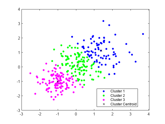
Generate a training data set using three distributions.
rng('default') % For reproducibility
X = [randn(100,2)*0.75+ones(100,2);
    randn(100,2)*0.5-ones(100,2);
    randn(100,2)*0.75];
Partition the training data into three clusters by using kmeans.
[idx,C] = kmeans(X,3);
Plot the clusters and the cluster centroids.
figure
gscatter(X(:,1),X(:,2),idx,'bgm')
hold on
plot(C(:,1),C(:,2),'kx')
legend('Cluster 1','Cluster 2','Cluster 3','Cluster Centroid')
Assign New Data to Existing Clusters
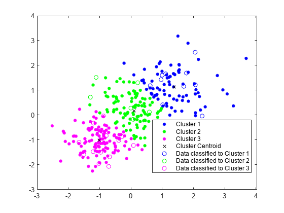
Generate a test data set.
Xtest = [randn(10,2)*0.75+ones(10,2);
    randn(10,2)*0.5-ones(10,2);
    randn(10,2)*0.75];
Classify the test data set using the existing clusters. Find the nearest centroid from each test data point by using pdist2.
[~,idx_test] = pdist2(C,Xtest,'euclidean','Smallest',1);
Plot the test data and label the test data using idx_test by using gscatter.
gscatter(Xtest(:,1),Xtest(:,2),idx_test,'bgm','ooo')
legend('Cluster 1','Cluster 2','Cluster 3','Cluster Centroid', ...
    'Data classified to Cluster 1','Data classified to Cluster 2', ...
    'Data classified to Cluster 3')
Generate Code
Generate C code that assigns new data to the existing clusters. Note that generating C/C++ code requires MATLAB® Coder™.
Define an entry-point function named findNearestCentroid that accepts centroid positions and new data, and then find the nearest cluster by using pdist2.
Add the %#codegen compiler directive (or pragma) to the entry-point function after the function signature to indicate that you intend to generate code for the MATLAB algorithm. Adding this directive instructs the MATLAB Code Analyzer to help you diagnose and fix violations that would cause errors during code generation.
type findNearestCentroid % Display contents of findNearestCentroid.m
function idx = findNearestCentroid(C,X) %#codegen
[~,idx] = pdist2(C,X,'euclidean','Smallest',1); % Find the nearest centroid
Note: If you click the button located in the upper-right section of this page and open this example in MATLAB®, then MATLAB® opens the example folder. This folder includes the entry-point function file.
Generate code by using codegen (MATLAB Coder). Because C and C++ are statically typed languages, you must determine the properties of all variables in the entry-point function at compile time. To specify the data type and array size of the inputs of findNearestCentroid, pass a MATLAB expression that represents the set of values with a certain data type and array size by using the -args option. For details, see Specify Variable-Size Arguments for Code Generation.
codegen findNearestCentroid -args {C,Xtest}
Code generation successful.
codegen generates the MEX function findNearestCentroid_mex with a platform-dependent extension.
Verify the generated code.
myIndx = findNearestCentroid(C,Xtest);
myIndex_mex = findNearestCentroid_mex(C,Xtest);
verifyMEX = isequal(idx_test,myIndx,myIndex_mex)
verifyMEX = logical
   1
isequal returns logical 1 (true), which means all the inputs are equal. The comparison confirms that the pdist2 function, the findNearestCentroid function, and the MEX function return the same index.
You can also generate optimized CUDA® code using GPU Coder™.
cfg = coder.gpuConfig('mex');
codegen -config cfg findNearestCentroid -args {C,Xtest}
For more information on code generation, see General Code Generation Workflow. For more information on GPU coder, see Get Started with GPU Coder (GPU Coder) and Supported Functions (GPU Coder).
The kmeans function ignores table rows that contain a missing value. To use all rows in the input data for k-means clustering, you can impute the missing values using a regression model.
Load the carbig data set and create a table that contains the Weight, Displacement, and Horsepower predictors.
load carbig
X = table(Weight,Displacement,Horsepower);
Display the number of missing values in each column of X.
MissingValues = sum(ismissing(X))
MissingValues = 1×3

     0     0     6
Column 3 (Horsepower) has six missing values. The other columns do not contain any missing values.
Train a multiple regression model using rows that do not contain missing values. Specify Horsepower as the response variable.
HPmodel = fitlm(rmmissing(X),"Horsepower");Display a plot of the regression model.
plot(HPmodel)

Impute the missing Horsepower values in X using the linear regression model.
imputedHP = predict(HPmodel,X(any(ismissing(X),2),1:2))
imputedHP = 6×1

   70.6749
  105.0360
   65.2328
   90.0460
   73.9490
   94.1612
Replace the missing Horsepower values with the imputed values.
X(any(ismissing(X),2),3) = table(imputedHP);
Cluster the data using k-means clustering. Specify that the data has three clusters.
[idx,C] = kmeans(table2array(X),3);
Plot the data and cluster assignments.
scatter3(X.Weight,X.Displacement,X.Horsepower,15,idx,"filled")
Input Arguments
Name-Value Arguments
Output Arguments
More About
Algorithms
kmeansuses a two-phase iterative algorithm to minimize the sum of point-to-centroid distances, summed over allkclusters.This first phase uses batch updates, where each iteration consists of reassigning points to their nearest cluster centroid, all at once, followed by recalculation of cluster centroids. This phase occasionally does not converge to solution that is a local minimum. That is, a partition of the data where moving any single point to a different cluster increases the total sum of distances. This is more likely for small data sets. The batch phase is fast, but potentially only approximates a solution as a starting point for the second phase.
This second phase uses online updates, where points are individually reassigned if doing so reduces the sum of distances, and cluster centroids are recomputed after each reassignment. Each iteration during this phase consists of one pass though all the points. This phase converges to a local minimum, although there might be other local minima with lower total sum of distances. In general, finding the global minimum is solved by an exhaustive choice of starting points, but using several replicates with random starting points typically results in a solution that is a global minimum.
If
Replicates= r > 1 andStartisplus(the default), then the software selects r possibly different sets of seeds according to the k-means++ algorithm.If you enable the
UseParalleloption inOptionsandReplicates> 1, then each worker selects seeds and clusters in parallel.
References
[1] Arthur, David, and Sergi Vassilvitskii. K-means++: The Advantages of Careful Seeding. In SODA ‘07: Proceedings of the Eighteenth Annual ACM-SIAM Symposium on Discrete Algorithms, 1027–1035. Society for Industrial and Applied Mathematics, 2007.
[2] Lloyd, S. Least Squares Quantization in PCM. IEEE Transactions on Information Theory 28, no. 2 (March 1982): 129–37.
[3] Seber, G. A. F. Multivariate Observations. Hoboken, NJ: John Wiley & Sons, Inc., 1984.
[4] Spath, H. Cluster Dissection and Analysis: Theory, FORTRAN Programs, Examples. Translated by J. Goldschmidt. New York: Halsted Press, 1985.
Extended Capabilities
Version History
Introduced before R2006a
See Also
linkage | clusterdata | incrementalKMeans | silhouette | parpool (Parallel Computing Toolbox) | statset | gmdistribution | kmedoids