simpleICP
simpleICP
This repo contains implementations of a rather simple version of the Iterative Closest Point (ICP) algorithm in various languages.
Currently, an implementation is available for:
| Language | Code | Main dependencies |
|---|---|---|
| C++ | Link | nanoflann, Eigen, cxxopts |
| Julia | Link | NearestNeighbors.jl |
| Matlab | Link | Statistics and Machine Learning Toolbox |
| Octave | Link | |
| Python | Link | NumPy, SciPy, lmfit, pandas |
I've tried to optimize the readability of the code, i.e. the code structure is as simple as possible and tests are rather rare.
The C++ version can be used through a cli interface.
Also available at:
Features of the ICP algorithm
Basic features
The following basic features are implemented in all languages:
-
Usage of the signed point-to-plane distance (instead of the point-to-point distance) as error metric. Main reasons:
-
Estimation of a rigid-body transformation (rotation + translation) for the movable point cloud. The final transformation is given as homogeneous transformation matrix H:
H = [R(0,0) R(0,1) R(0,2)   tx]
    [R(1,0) R(1,1) R(1,2)   ty]
    [R(2,0) R(2,1) R(2,2)   tz]
    [     0      0      0    1]
where
Ris the rotation matrix andtx,ty, andtzare the components of the translation vector. UsingH, the movable point cloud can be transformed with:Xt = H*Xwhere
Xis a 4-by-n matrix holding in each column the homogeneous coordinatesx,y,z,1of a single point, andXtis the resulting 4-by-n matrix with the transformed points. -
Selection of a fixed number of correspondences between the fixed and the movable point cloud. Default is
correspondences = 1000. -
Automatic rejection of potentially wrong correspondences on the basis of
- the median of absolute deviations. A correspondence
iis rejected if|dist_i-median(dists)| > 3*sig_mad, wheresig_mad = 1.4826*mad(dists). - the planarity of the plane used to estimate the normal vector (see below). The planarity is defined as
P = (ev2-ev3)/ev1(ev1 >= ev2 >= ev3), whereevare the eigenvalues of the covariance matrix of the points used to estimate the normal vector. A correspondenceiis rejected ifP_i < min_planarity. Default ismin_planarity = 0.3.
- the median of absolute deviations. A correspondence
-
After each iteration a convergence criteria is tested: if the mean and the standard deviation of the point-to-plane distances do not change more than
min_changepercent, the iteration is stopped. Default ismin_change = 1. -
The normal vector of the plane (needed to compute the point-to-plane distance) is estimated from the fixed point cloud using a fixed number of neighbors. Default is
neighbors = 10. -
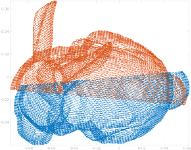
The point clouds must not fully overlap, i.e. a partial overlap of the point cloud is allowed. An example for such a case is the Bunny dataset, see here. The initial overlapping area between two point clouds can be defined by the parameter
max_overlap_distance. More specifically, the correspondences are only selected across points of the fixed point cloud for which the initial distance to the nearest neighbor of the movable point cloud is<= max_overlap_distance.
Extended features
The extended features are currently not implemented in all languages. The differences are documented in the following table:
| Feature | C++ | Julia | Matlab | Octave | Python |
|---|---|---|---|---|---|
| observation of rigid-body transformation parameters | no | no | no | no | yes |
Extended feature: observation of rigid-body transformation parameters
This is useful in at least these cases:
-
If only a subset of the 6 rigid-body transformation parameters should be estimated. This can be accomplished by setting the weight of individual parameters to infinite, see example below.
-
If all or a subset of the 6 rigid-body transformation parameters have been directly observed in any other way, e.g. by means of a manual measurement.
-
If estimates for the rigid-body transformation parameters exist, e.g. from a previous run of simpleICP. In this case the observation weight should be set (according to the theory of least squares adjustments) to
w = 1/observation_error^2whereby theobservation_erroris defined asstd(observation_value). The observation error of all parameters is reported by simpleICP as "est.uncertainty" in the logging output.
This feature introduces two new parameters: rbp_observed_values and rbp_observation_weights. Both parameters have exactly 6 elements which correspond to the rigid-body transformation parameters in the following order:
-
alpha1: rotation angle around the x-axis -
alpha2: rotation angle around the y-axis -
alpha3: rotation angle around the z-axis -
tx: x component of translation vector -
ty: y component of translation vector -
tz: z component of translation vector
The rigid-body transformation is defined in non-homogeneous coordinates as follows:
Xt = RX + t
where X and Xt are n-by-3 matrices of the original and transformed movable point cloud, resp., t is the translation vector, and R the rotation matrix. R is thereby defined as:
R = [ca2*ca3               -ca2*sa3                sa2    ]
    [ca1*sa3+sa1*sa2*ca3    ca1*ca3-sa1*sa2*sa3   -sa1*ca2]
    [sa1*sa3-ca1*sa2*ca3    sa1*ca3+ca1*sa2*sa3    ca1*ca2]
with the substitutions:
sa1 := sin(alpha1), ca1 := cos(alpha1)
sa2 := sin(alpha2), ca2 := cos(alpha2)
sa3 := sin(alpha3), ca3 := cos(alpha3)
The two parameters rbp_observed_values and rbp_observation_weights can be used to introduce an additional observation to the least squares optimization for each transformation parameter:
residual = observation_weight * (estimated_value - observed_value)
Example which demonstrates the most important combinations:
# parameters:              alpha1   alpha2   alpha3   tx      ty     tz
rbp_observed_values =     (10.0     0.0     -5.0      0.20   -0.15   0.0)
rbp_observation_weights = (100.0    0.0      0.0      40.0    40.0   inf)
Consequently:
-
alpha1: is observed to be 10 degrees with an observation weight of 100. -
alpha2: is not observed since the corresponding weight is zero. However, the observed value is used as initial value foralpha2in the non-linear least squares optimization. -
alpha3: is also not observed, but has an initial value of -5 degrees. -
tx: is observed to be 0.20 with an observation weight of 40. -
ty: is observed to be -0.15 with an observation weight of 40. -
tz: is observed to be 0 with an infinite observation weight, i.e. this parameter becomes a constant and is fixed to be exactly the observation value. Thus, in this case only 5 (out of 6) rigid-body transformation parameters are estimated.
Output
All implementations generate the same screen output. This is an example from the C++ version for the Bunny dataset:
$ run_simpleicp.sh
Processing dataset "Dragon"
Create point cloud objects ...
Select points for correspondences in fixed point cloud ...
Estimate normals of selected points ...
Start iterations ...
Iteration | correspondences | mean(residuals) |  std(residuals)
   orig:0 |             767 |          0.0001 |          0.3203
        1 |             767 |         -0.0061 |          0.2531
        2 |             773 |         -0.0035 |          0.1669
        3 |             771 |         -0.0008 |          0.0835
        4 |             741 |         -0.0006 |          0.0196
        5 |             762 |          0.0000 |          0.0025
        6 |             775 |          0.0001 |          0.0022
Convergence criteria fulfilled -> stop iteration!
Estimated transformation matrix H:
[    0.998696     0.052621    -0.034179    -0.206737]
[   -0.052090     0.999028     0.020119    -0.408088]
[    0.034822    -0.018663     0.999436    -0.593361]
[    0.000000     0.000000     0.000000     1.000000]
Finished in 1.729 seconds!
Test data sets
The test data sets are included in the data subfolder. An example call for each language can be found in the run_simpleicp.* files, e.g. run_simpleicp.jl for the julia version.
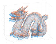
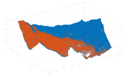
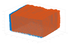
| Dataset | pc1 (no_pts) | pc2 (no_pts) | Overlap | Source | |
|---|---|---|---|---|---|
| Dragon |  |
pc1 (100k) | pc2 (100k) | full overlap | The Stanford 3D Scanning Repository |
| Airborne Lidar |  |
pc1 (1340k) | pc2 (1340k) | full overlap | Airborne Lidar flight campaign over Austrian Alps |
| Terrestrial Lidar |  |
pc1 (1250k) | pc2 (1250k) | full overlap | Terrestrial Lidar point clouds of a stone block |
| Bunny |  |
pc1 (21k) | pc2 (22k) | partial overlap | The Stanford 3D Scanning Repository |
Benchmark
These are the runtimes on my PC for the data sets above:
| Dataset | C++ | Julia | Matlab | Octave* | Python |
|---|---|---|---|---|---|
| Dragon | 0.16s | 3.99s | 1.34s | 95.7s | 4.51s |
| Airborne Lidar | 3.98s | 5.38s | 15.08s | - | 16.49s |
| Terrestrial Lidar | 3.62s | 5.22s | 13.24s | - | 14.45s |
| Bunny | 0.13s | 0.38s | 0.37s | 72.8s | 4.20s |
For all versions the same input parameters (correspondences, neighbors, ...) are used.
* Unfortunately, I haven't found an implementation of a kd tree in Octave (it is not yet implemented in the Statistics package). Thus, a (very time-consuming!) exhaustive nearest neighbor search is used instead. For larger datasets the Octave timings are missing, as the distance matrix does not fit into memory.
References
Please cite related papers if you use this code:
@article{glira2015a,
  title={A Correspondence Framework for ALS Strip Adjustments based on Variants of the ICP Algorithm},
  author={Glira, Philipp and Pfeifer, Norbert and Briese, Christian and Ressl, Camillo},
  journal={Photogrammetrie-Fernerkundung-Geoinformation},
  volume={2015},
  number={4},
  pages={275--289},
  year={2015},
  publisher={E. Schweizerbart'sche Verlagsbuchhandlung}
}
Related projects
- globalICP: A multi-scan ICP implementation for Matlab
Star History
Cite As
Glira, Philipp, et al. “A Correspondence Framework for ALS Strip Adjustments Based on Variants of the ICP Algorithm.” Photogrammetrie - Fernerkundung - Geoinformation, vol. 2015, no. 4, Schweizerbart, Aug. 2015, pp. 275–89, doi:10.1127/pfg/2015/0270.
MATLAB Release Compatibility
Platform Compatibility
Windows macOS LinuxTags
Community Treasure Hunt
Find the treasures in MATLAB Central and discover how the community can help you!
Start Hunting!Discover Live Editor
Create scripts with code, output, and formatted text in a single executable document.
data
matlab
octave
| Version | Published | Release Notes | |
|---|---|---|---|
| 1.0 |


