Classify crack image using deep learning and explain "WHY"
Classify crack images and explain why using MATLAB
[English]
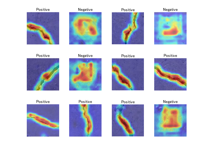
This demo shows how to fine-tune a pretrained deep convolutional network called SqueezeNet [1] to perform a crack/normal image classification. The classification output was discussed using a technique to "explain why" called grad-cam as shown below. This script was created based on the official documentation [2]. For the grad-cam, I referred to [3]. About fine-tuning, please refer to the additional explanation [a] at the end of this script. In this demo, we use a dataset of concrete crack images introduced by L. Zhang [4]. The data is available at [5].
[Japanese]
この例では、深層学習を用いて、ひび割れ画像を分類するコードを示します。あらかじめ大規模な画像のデータセットで学習し、よい画像の特徴を捉えられる事前学習ネットワークを用いて、その構造をもとに学習したり、その重み初期値として利用します。また、grad-camとよばれる手法を用いて、分類の際に重要視された領域を可視化します。この例では、事前学習ネットワークの中でも非常にサイズの小さい、SqueezeNet [1] を用います。また、本デモでは、[2] [3]にある、公式ドキュメントを参考にしました。データセットは、[4]の論文で紹介されているデータセット [5]を用いました。
[Key words]
class activation mapping, classification, crack, deep learning, explainable, grad-cam
[2] Matlab Documentation: Train Deep Learning Network to Classify New Images
[3] Matlab Documentation: Grad-CAM Reveals the Why Behind Deep Learning Decisions
[5] Concrete Crack Images for Classification
Load Data
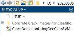
First of all, please download "Concrete Crack Images for Classification" from [4]. Then unzip it to name as Concrete Crack Images for Classification. Please run this code after confirming that the file is in your current directory as shown below.
Use imageDatastore function to store images with the label information. The label information was recognized based on the folder name in the file, Concrete Crack Images for Classification.
clear;clc;close all
imds = imageDatastore('Concrete Crack Images for Classification','IncludeSubfolders',true, 'LabelSource','foldernames');
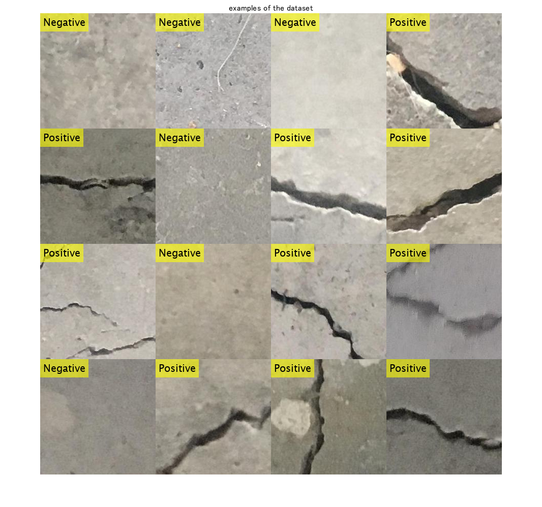
This dataset contains normal (Negative) and crack images (Positive). Display some sample images.
numExample=16;
idx = randperm(numel(imds.Files),numExample);
for i=1:numExample
    I=readimage(imds,idx(i));
    I_tile{i}=insertText(I,[1,1],string(imds.Labels(idx(i))),'FontSize',20);
end
% use imtile function to tile out the example images
I_tile = imtile(I_tile);
figure;imshow(I_tile);title('examples of the dataset')
Dividing images
Divide the data into training, validation and test data sets. The function splitEachLabel splits the images datastore into two new datastores. This dataset contains 20k normal images and 20k crack images. As the dataset has numerous images, it takes some time to train. Just for enjoying this demo, you can set the ratio for training images low, such as 0.1 to get the number of images very small.
The ratio after imds represets the ratio with which the number of images for train, validation and test data are determined.
For example, if the ratio is 0.1, the number of images is 40k*0.1=4000.
[imdsTrain,imdsValidation,imdsTest] = splitEachLabel(imds,0.1,0.1,0.1,'randomized');
Count the number of images in the training dataset. Confirm if the number is as expected from above.
numTrainImages = numel(imdsTrain.Labels)
numTrainImages = 4000
Load Pretrained Network
Load the pretrained SqueezeNet neural network. Squeezenet is the smallest pre-trained network among the networks available officially supported by Matlab.
net = squeezenet;
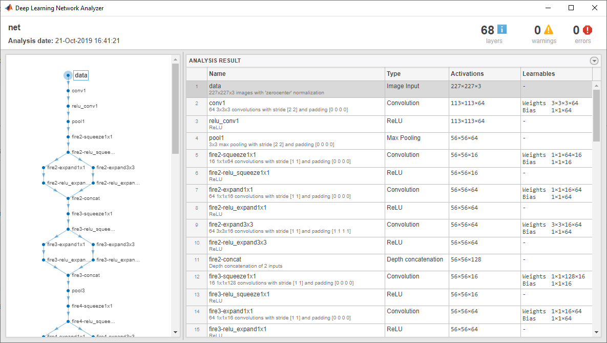
Use analyzeNetwork to display an interactive visualization of the network architecture and detailed information about the network layers.
analyzeNetwork(net)
The first layer, the image input layer, requires input images of size 227-by-227-by-3, where 3 is the number of color channels.
inputSize = net.Layers(1).InputSize
inputSize = 1x3
   227   227     3
Replace Final Layers
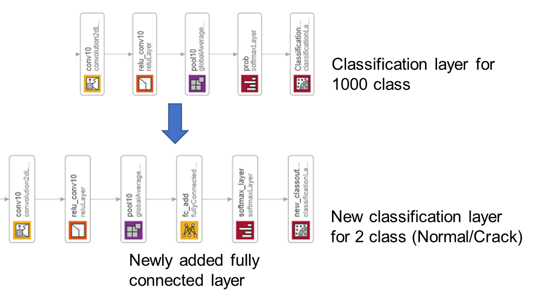
As the original version of the SqueezeNet is a network for 1000 classes, we have to adapt it to normal/crack classification (2-classes).
Extract the layer graph from the trained network.
lgraph = layerGraph(net);
In most networks, the last layer with learnable weights is a fully connected layer. In some networks, such as SqueezeNet, the last learnable layer is a 1-by-1 convolutional layer instead. In this case, we added a fully connected layer before softmax layer.
numClasses = numel(categories(imdsTrain.Labels))
numClasses = 2
Remove the classification layer for 1000 classes and relace it by the new layers for our task.
newlgraph = removeLayers(lgraph,{'ClassificationLayer_predictions'});
lgraph = replaceLayer(newlgraph,'prob',[fullyConnectedLayer(numClasses,'Name','fc_add');softmaxLayer('Name','softmax_layer'); classificationLayer('Name','new_classoutput')]);
The classification layer specifies the output classes of the network. Replace the classification layer with a new one without class labels. trainNetwork automatically sets the output classes of the layer at training time.
Prepare for augmentation
The network requires input images of size 227-by-227-by-3, but the images in the image datastores have different sizes. Use an augmented image datastore to automatically resize the training images. Specify additional augmentation operations to perform on the training images: randomly flip the training images along the vertical axis, and randomly translate them up to 30 pixels horizontally and vertically. Data augmentation helps prevent the network from overfitting and memorizing the exact details of the training images.
pixelRange = [-30 30];
imageAugmenter = imageDataAugmenter( ...
    'RandXReflection',true, ...
    'RandXTranslation',pixelRange, ...
    'RandYTranslation',pixelRange);
augimdsTrain = augmentedImageDatastore(inputSize(1:2),imdsTrain, ...
    'DataAugmentation',imageAugmenter);
To automatically resize the validation and test images without performing further data augmentation, use an augmented image datastore without specifying any additional preprocessing operations.
augimdsValidation = augmentedImageDatastore(inputSize(1:2),imdsValidation);
augimdsTest = augmentedImageDatastore(inputSize(1:2),imdsTest);
Train Network
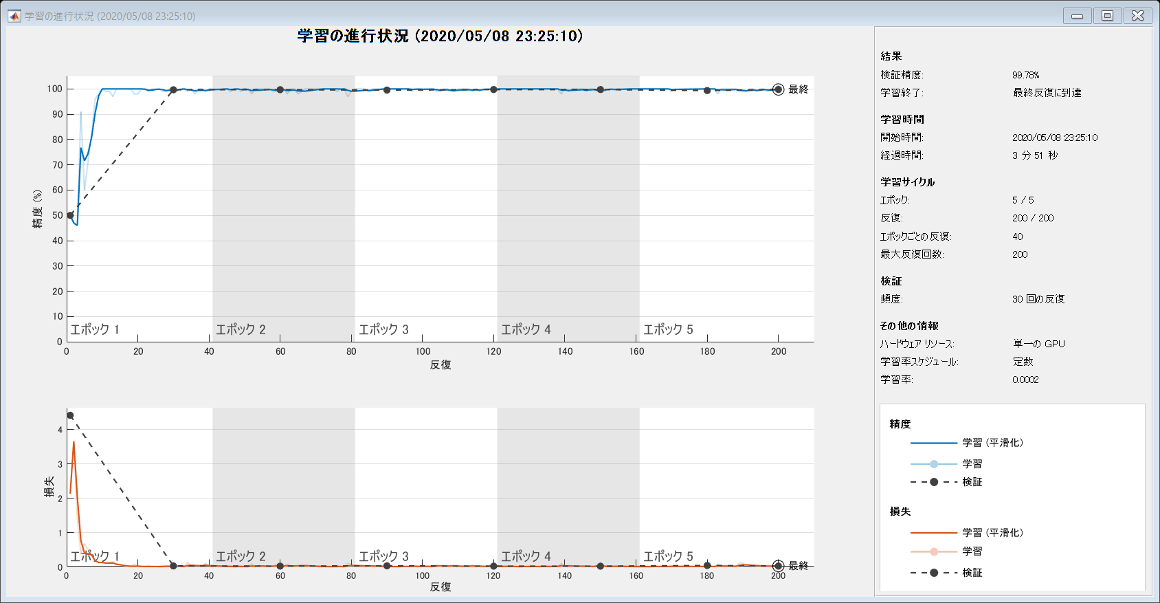
Specify the training options. As an optimizer, we use adam optimizer.
options = trainingOptions('adam', ...
    'MiniBatchSize',100, ...
    'MaxEpochs',5, ...
    'InitialLearnRate',2e-4, ...
    'Shuffle','every-epoch', ...
    'ValidationData',augimdsValidation, ...
    'ExecutionEnvironment',"auto", ...
    'ValidationFrequency',30, ...
    'Verbose',false, ...
    'Plots','training-progress');
The network is trained on GPU if available. It is specified by ExecutionEnvironment,"auto" as above.
netTransfer = trainNetwork(augimdsTrain,lgraph,options);
Classify test Images to calculate the classification accuracy
Classify the test images of the normal and crack images using the fine-tuned network.
You can use classify function to classify the images using a network.
[YPred,scores] = classify(netTransfer,augimdsTest);
Display four sample validation images with their predicted labels.
Calculate the classification accuracy on the validation set. Accuracy is the fraction of labels that the network predicts correctly.
YTest = imdsTest.Labels;
accuracy = mean(YPred == YTest)
accuracy = 0.9978
Explore "why" using grad-cam
For the detail of grad-cam, please refer to Matlab Documentation: Grad-CAM Reveals the Why Behind Deep Learning Decisions.
lgraph = layerGraph(netTransfer);
To access the data that SqueezeNet uses for classification, remove its final classification layer.
lgraph = removeLayers(lgraph, lgraph.Layers(end).Name);
Create a dlnetwork from the layer graph.
dlnet = dlnetwork(lgraph);
Specify the name for Grad-cam.
softmaxName = 'softmax_layer';
featureLayerName = 'relu_conv10';
dispNum controls the number of images to use grad-cam.
dispNum=12;
idx = randperm(numel(imdsTest.Files),dispNum);
C=cell(dispNum,1);
figure
for i = 1:dispNum
img = readimage(imdsValidation,idx(i));

[classfn,~] = classify(netTransfer,img);
To use automatic differentiation, convert the sherlock image to a dlarray.
dlImg = dlarray(single(img),'SSC');
Compute the Grad-CAM gradient for the image by calling dlfeval on the gradcam function.
[featureMap, dScoresdMap] = dlfeval(@gradcam, dlnet, dlImg, softmaxName, featureLayerName, classfn);
Resize the gradient map to the SqueezeNet image size, and scale the scores to the appropriate levels for display.
gradcamMap = sum(featureMap .* sum(dScoresdMap, [1 2]), 3);
gradcamMap = extractdata(gradcamMap);
gradcamMap = rescale(gradcamMap);
subplot(3,4,i)
imshow(img);title(classfn)
hold on;
subplot(3,4,i)
imagesc(imresize(gradcamMap,inputSize(1:2) ,'Method', 'bicubic'),'AlphaData',0.5);
colormap jet
hold off;
end
Show the Grad-CAM levels on top of the image by using an 'AlphaData' value of 0.5. The 'jet' colormap has deep blue as the lowest value and deep red as the highest.
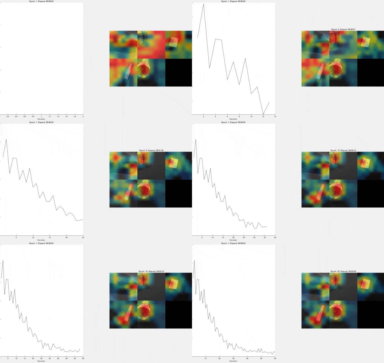
This kind of visualization to show where is important for the classification can be done during the traing process, too. We can confirm that the network graducally learns a good feature for the classification. For the demo, please look here.
Kenta (2020). Continuous activation map generation at training process (https://www.github.com/giants19/Continuous-class-activation-generation-during-training-process-using-Matlab), GitHub. Retrieved May 8, 2020.
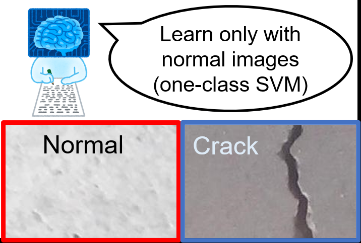
If the number of anomaly images is totally limited, you can learn only with normal images using, for example, one-class SVM.
For the demo, please check here.
Helper function
function [featureMap,dScoresdMap] = gradcam(dlnet, dlImg, softmaxName, featureLayerName, classfn)
[scores,featureMap] = predict(dlnet, dlImg, 'Outputs', {softmaxName, featureLayerName});
classScore = scores(classfn);
dScoresdMap = dlgradient(classScore,featureMap);
end
Additional explanations
[a] SqueezeNet has been trained on over a million images and can classify images into 1000 object categories (such as keyboard, coffee mug, pencil, and many animals). The network has learned rich feature representations for a wide range of images. The network takes an image as input and outputs a label for the object in the image together with the probabilities for each of the object categories (cited from the official document).
[b] Transfer learning is commonly used in deep learning applications. You can take a pretrained network and use it as a starting point to learn a new task. Fine-tuning a network with transfer learning is usually much faster and easier than training a network with randomly initialized weights from scratch. You can quickly transfer learned features to a new task using a smaller number of training images (cited from the official document).
Cite As
Kenta (2024). Classify crack image using deep learning and explain "WHY" (https://github.com/KentaItakura/Classify-crack-image-and-explain-why-using-MATLAB/releases/tag/v1.1), GitHub. Retrieved .
MATLAB Release Compatibility
Platform Compatibility
Windows macOS LinuxCategories
Tags
Community Treasure Hunt
Find the treasures in MATLAB Central and discover how the community can help you!
Start Hunting!Discover Live Editor
Create scripts with code, output, and formatted text in a single executable document.
plainCode
| Version | Published | Release Notes | |
|---|---|---|---|
| 1.1 | See release notes for this release on GitHub: https://github.com/KentaItakura/Classify-crack-image-and-explain-why-using-MATLAB/releases/tag/v1.1 |
||
| 1.0.1 | keywords added |
||
| 1.0.0 |
