kernel density estimation
fast and accurate state-of-the-art bivariate kernel density estimator with diagonal bandwidth matrix.
The kernel is assumed to be Gaussian. The two bandwidth parameters are chosen optimally without ever
using/assuming a parametric model for the data or any "rules of thumb". Unlike many other procedures, this one
is immune to accuracy failures in the estimation of multimodal densities with widely separated modes (see examples).
INPUTS:
data - an N by 2 array with continuous data
n - size of the n by n grid over which the density is computed
n has to be a power of 2, otherwise n=2^ceil(log2(n)); the default value is 2^8;
MIN_XY,MAX_XY - limits of the bounding box over which the density is computed;
the format is:
MIN_XY=[lower_Xlim,lower_Ylim]
MAX_XY=[upper_Xlim,upper_Ylim].
The dafault limits are computed as:
MAX=max(data,[],1); MIN=min(data,[],1); Range=MAX-MIN;
MAX_XY=MAX+Range/4; MIN_XY=MIN-Range/4;
OUTPUT:
bandwidth - a row vector with the two optimal bandwidths for a bivaroate Gaussian kernel;
the format is:
bandwidth=[bandwidth_X, bandwidth_Y];
density - an 'n' by 'n' matrix containing the density values over the 'n' by 'n' grid;
density is not computed unless the function is asked for such an output;
X,Y - the meshgrid over which the variable "density" has been computed;
the intended usage is as follows:
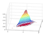
surf(X,Y,density)
Example (simple Gaussian mixture)
clear all
% generate a Gaussian mixture with distant modes
data=[randn(500,2);
randn(500,1)+3.5, randn(500,1);];
% call the routine
[bandwidth,density,X,Y]=kde2d(data);
% plot the data and the density estimate
contour3(X,Y,density,50), hold on
plot(data(:,1),data(:,2),'r.','MarkerSize',5)
Example (Gaussian mixture with distant modes):
clear all
% generate a Gaussian mixture with distant modes
data=[randn(100,1), randn(100,1)/4;
randn(100,1)+18, randn(100,1);
randn(100,1)+15, randn(100,1)/2-18;];
% call the routine
[bandwidth,density,X,Y]=kde2d(data);
% plot the data and the density estimate
surf(X,Y,density,'LineStyle','none'), view([0,60])
colormap hot, hold on, alpha(.8)
set(gca, 'color', 'blue');
plot(data(:,1),data(:,2),'w.','MarkerSize',5)
Example (Sinusoidal density):
clear all
X=rand(1000,1); Y=sin(X*10*pi)+randn(size(X))/3; data=[X,Y];
% apply routine
[bandwidth,density,X,Y]=kde2d(data);
% plot the data and the density estimate
surf(X,Y,density,'LineStyle','none'), view([0,70])
colormap hot, hold on, alpha(.8)
set(gca, 'color', 'blue');
plot(data(:,1),data(:,2),'w.','MarkerSize',5)
Reference:
Kernel density estimation via diffusion
Z. I. Botev, J. F. Grotowski, and D. P. Kroese (2010)
Annals of Statistics, Volume 38, Number 5, pages 2916-2957
doi:10.1214/10-AOS799
Cite As
Zdravko Botev (2026). kernel density estimation (https://nl.mathworks.com/matlabcentral/fileexchange/17204-kernel-density-estimation), MATLAB Central File Exchange. Retrieved .
MATLAB Release Compatibility
Platform Compatibility
Windows macOS LinuxCategories
Tags
Acknowledgements
Inspired: synctest( X,varargin ), Cornerplot, Kernel Density Estimator for High Dimensions
Discover Live Editor
Create scripts with code, output, and formatted text in a single executable document.
| Version | Published | Release Notes | |
|---|---|---|---|
| 1.3.0.0 | The algorithm uses the FFT for speed. Sometimes round-off computational errors due to using the FFT result in vanishingly small density values (e.g. -10^-17). Any such values are now set to machine precision.
|
||
| 1.2.0.0 | updated reference and added new license as requested by Matlab |
||
| 1.0.0.0 |

