fourier-neural-operator
Fourier Neural Operator
The Fourier Neural Operator (FNO) [1] is a neural operator with an integral kernel parameterized in Fourier space. This allows for an expressive and efficient architecture. Applications of the FNO include weather forecasting and, more generically, finding efficient solutions to the Navier-Stokes equations which govern fluid flow.
Setup
Add fno directory to the path.
addpath(genpath('fno'));Requirements
Requires:
- MATLAB (R2021b or newer)
- Deep Learning Toolbox™
References
[1] Zongyi Li, Nikola Kovachki, Kamyar Azizzadenesheli, Burigede Liu, Kaushik Bhattacharya, Andrew Stuart, and Anima Anandkumar. Fourier Neural Operator for Parametric Partial Differential Equations. In International Conference on Learning Representations (ICLR), 2021a. (https://openreview.net/forum?id=c8P9NQVtmnO)
Example: Fourier Neural Operator for 1d Burgers' Equation
In this example we apply the Fourier Neural Operator to learn the one-dimensional Burgers' equation with the following definition:
where and
is the Reynolds number. Periodic boundary conditions are imposed across the spatial domain. We learn the operator mapping the initial condition
to the solution at time
:
.
Data preparation
We use the burgers_data_R10.mat, which contains initial velocities and solutions
of the Burgers' equation. We then use these as training inputs and targets respectively. The network inputs include the spatial domain
at the desired discretization. In this example we choose a grid size of
.
% Setup.
addpath(genpath('fno'));

% Download training data.
dataDir = fullfile('data');
if ~isfolder(dataDir)
    mkdir(dataDir);
end
dataFile = fullfile(dataDir,'burgers_data_R10.mat');
if ~exist(dataFile, 'file')
    location = 'https://ssd.mathworks.com/supportfiles/nnet/data/burgers1d/burgers_data_R10.mat';
    websave(dataFile, location);
end
data = load(dataFile, 'a', 'u');
x = data.a;
t = data.u;

% Specify the number of observations in training and test data, respectively.
numTrain = 1e3;
numTest = 1e2;

% Specify grid size and downsampling factor.
h = 2^10;
n = size(x,2);
ns = floor(n./h);

% Downsample the data for training.
xTrain = x(1:numTrain, 1:ns:n);
tTrain = t(1:numTrain, 1:ns:n);
xTest = x(end-numTest+1:end, 1:ns:n);
tTest = t(end-numTest+1:end, 1:ns:n);

% Define the grid over the spatial domain x.
xmax = 1;
xgrid = linspace(0, xmax, h);

% Combine initial velocities and spatial grid to create network
% predictors.
xTrain = cat(3, xTrain, repmat(xgrid, [numTrain 1]));
xTest = cat(3, xTest, repmat(xgrid, [numTest 1]));
Define network architecture
Here we create a dlnetwork for the Burgers' equation problem. The network accepts inputs of dimension [h 2 miniBatchSize], and returns outputs of dimension [h 1 miniBatchSize]. The network consists os multiple blocks which combine spectral convolution with regular, linear convolution. The convolution in Fourier space filters out higher order oscillations in the solution, while the linear convolution learns local correlations.
numModes = 16;
width = 64;

lg = layerGraph([ ...
    convolution1dLayer(1, width, Name='fc0')

    spectralConvolution1dLayer(width, numModes, Name='specConv1')
    additionLayer(2, Name='add1')
    reluLayer(Name='relu1')

    spectralConvolution1dLayer(width, numModes, Name='specConv2')
    additionLayer(2, Name='add2')
    reluLayer(Name='relu2')

    spectralConvolution1dLayer(width, numModes, Name='specConv3')
    additionLayer(2, Name='add3')
    reluLayer(Name='relu3')

    spectralConvolution1dLayer(width, numModes, Name='specConv4')
    additionLayer(2, Name='add4')

    convolution1dLayer(1, 128, Name='fc5')
    reluLayer(Name='relu5')
    convolution1dLayer(1, 1, Name='fc6')
    ]);

lg = addLayers(lg, convolution1dLayer(1, width, Name='fc1'));
lg = connectLayers(lg, 'fc0', 'fc1');
lg = connectLayers(lg, 'fc1', 'add1/in2');

lg = addLayers(lg, convolution1dLayer(1, width, Name='fc2'));
lg = connectLayers(lg, 'relu1', 'fc2');
lg = connectLayers(lg, 'fc2', 'add2/in2');

lg = addLayers(lg, convolution1dLayer(1, width, Name='fc3'));
lg = connectLayers(lg, 'relu2', 'fc3');
lg = connectLayers(lg, 'fc3', 'add3/in2');

lg = addLayers(lg, convolution1dLayer(1, width, Name='fc4'));
lg = connectLayers(lg, 'relu3', 'fc4');
lg = connectLayers(lg, 'fc4', 'add4/in2');

numInputChannels = 2;
XInit = dlarray(ones([h numInputChannels 1]), 'SCB');
net = dlnetwork(lg, XInit);

analyzeNetwork(net)
Training options
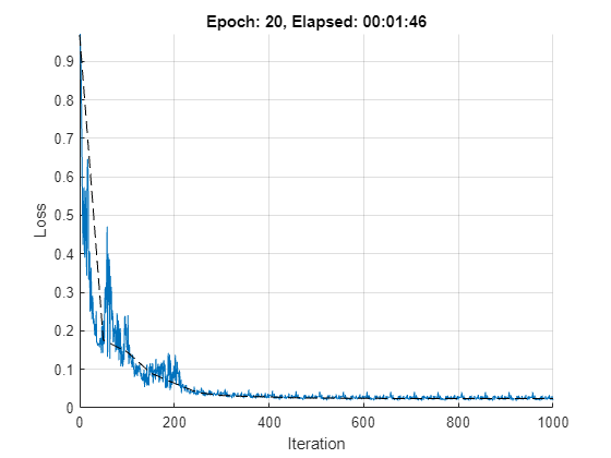
The network is trained using the standard SGDM algorithm, where the learn rate is decreased every stepSize iterations.
executionEnvironment = "gpu";

batchSize = 20;
learnRate = 1e-3;
momentum = 0.9;

numEpochs = 20;
stepSize = 100;
gamma = 0.5;
expNum = 1;
checkpoint = false;
expDir = sprintf( 'checkpoints/run%g', expNum );
if ~isfolder( expDir ) && checkpoint
    mkdir(expDir)
end

vel = [];
totalIter = 0;

numTrain = size(xTrain,1);
numIterPerEpoch = floor(numTrain./batchSize);
Training loop
Train the network.
if executionEnvironment == "gpu" && canUseGPU
    xTrain = gpuArray(xTrain);
    xTest = gpuArray(xTest);
end

start = tic;
figure;
clf
lineLossTrain = animatedline('Color', [0 0.4470 0.7410]);
lineLossTest = animatedline('Color', 'k', 'LineStyle', '--');
ylim([0 inf])
xlabel("Iteration")
ylabel("Loss")
grid on

% Compute initial validation loss.
y = net.predict( dlarray(xTest, 'BSC') );
yTest = extractdata(permute(stripdims(y), [3 1 2]));
relLossTest = relativeL2Loss(yTest , tTest);
addpoints(lineLossTest, 0, double(relLossTest/size(xTest,1)))

% Main loop.
lossfun = dlaccelerate(@modelLoss);
for epoch = 1:numEpochs
    % Shuffle the data.
    dataIdx = randperm(numTrain);

    for iter = 1:numIterPerEpoch
        % Get mini-batch data.
        batchIdx = (1:batchSize) + (iter-1)*batchSize;
        idx = dataIdx(batchIdx);
        X = dlarray( xTrain(batchIdx, :, :), 'BSC' );
        T = tTrain(batchIdx, :);

        % Compute loss and gradients.
        [loss, dnet] = dlfeval(lossfun, X, T, net);

        % Update model parameters using SGDM update rule.
        [net, vel] = sgdmupdate(net, dnet, vel, learnRate, momentum);

        % Plot training progress.
        totalIter = totalIter + 1;
        D = duration(0,0,toc(start),'Format','hh:mm:ss');
        addpoints(lineLossTrain,totalIter,double(extractdata(loss/batchSize)))
        title("Epoch: " + epoch + ", Elapsed: " + string(D))
        drawnow

        % Learn rate scheduling.
        if mod(totalIter, stepSize) == 0
            learnRate = gamma.*learnRate;
        end
    end
    % Compute validation loss and MSE.
    y = net.predict( dlarray(xTest, 'BSC') );
    yTest = extractdata(permute(stripdims(y), [3 1 2]));
    relLossTest = relativeL2Loss( yTest , tTest );
    mseTest = mean( (yTest(:) - tTest(:)).^2 );

    % Display progress.
    D = duration(0,0,toc(start),'Format','hh:mm:ss');
    numTest = size(xTest, 1);
    fprintf('Epoch = %g, train loss = %g, val loss = %g, val mse = %g, total time = %s. \n', ...
        epoch, extractdata(loss)/batchSize, relLossTest/numTest, mseTest/numTest, string(D));
    addpoints(lineLossTest, totalIter, double(relLossTest/numTest))

    % Checkpoints.
    if checkpoint
        filename = sprintf('checkpoints/run%g/epoch%g.mat', expNum, epoch);
        save(filename, 'net', 'epoch', 'vel', 'totalIter', 'relLossTest', 'mseTest', 'learnRate');
    end
end
Epoch = 1, train loss = 0.226405, val loss = 0.175389, val mse = 7.73286e-05, total time = 00:00:13.
Epoch = 2, train loss = 0.153691, val loss = 0.145805, val mse = 5.99213e-05, total time = 00:00:22.
Epoch = 3, train loss = 0.0923258, val loss = 0.0904608, val mse = 2.49174e-05, total time = 00:00:27.
Epoch = 4, train loss = 0.102122, val loss = 0.0639219, val mse = 1.43723e-05, total time = 00:00:32.
Epoch = 5, train loss = 0.0346076, val loss = 0.0393621, val mse = 9.33419e-06, total time = 00:00:36.
Epoch = 6, train loss = 0.0361029, val loss = 0.032303, val mse = 7.10724e-06, total time = 00:00:45.
Epoch = 7, train loss = 0.0270364, val loss = 0.0296161, val mse = 6.43696e-06, total time = 00:00:50.
Epoch = 8, train loss = 0.0263171, val loss = 0.0283881, val mse = 5.92292e-06, total time = 00:00:54.
Epoch = 9, train loss = 0.0248211, val loss = 0.0261364, val mse = 5.54218e-06, total time = 00:00:58.
Epoch = 10, train loss = 0.0243392, val loss = 0.0253596, val mse = 5.32946e-06, total time = 00:01:03.
Epoch = 11, train loss = 0.0236119, val loss = 0.0250861, val mse = 5.22886e-06, total time = 00:01:07.
Epoch = 12, train loss = 0.023318, val loss = 0.024752, val mse = 5.12552e-06, total time = 00:01:11.
Epoch = 13, train loss = 0.0230901, val loss = 0.0243369, val mse = 5.04185e-06, total time = 00:01:16.
Epoch = 14, train loss = 0.0229644, val loss = 0.0241713, val mse = 4.99882e-06, total time = 00:01:20.
Epoch = 15, train loss = 0.0228391, val loss = 0.0240904, val mse = 4.99516e-06, total time = 00:01:25.
Epoch = 16, train loss = 0.022768, val loss = 0.0240143, val mse = 4.97173e-06, total time = 00:01:29.
Epoch = 17, train loss = 0.0228152, val loss = 0.023916, val mse = 4.95474e-06, total time = 00:01:33.
Epoch = 18, train loss = 0.022787, val loss = 0.0238792, val mse = 4.94643e-06, total time = 00:01:38.
Epoch = 19, train loss = 0.0227602, val loss = 0.023865, val mse = 4.93665e-06, total time = 00:01:42.
Epoch = 20, train loss = 0.0227464, val loss = 0.0238451, val mse = 4.93358e-06, total time = 00:01:46.
Test on unseen, higher resolution data
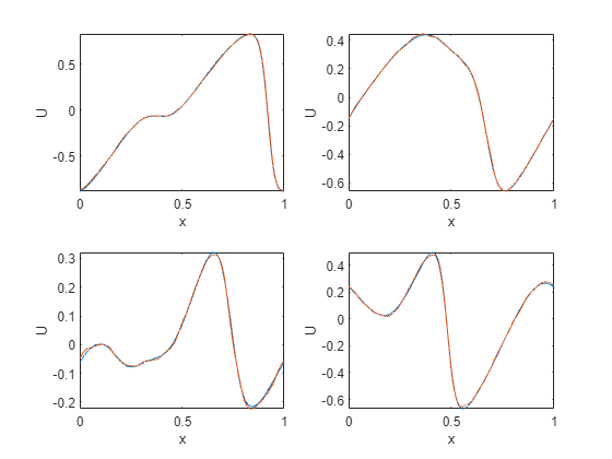
Here we take the trained network and test on unseen data with a higher spatial resolution than the training data. This is an example of zero-shot super-resolution.
gridHighRes = linspace(0, xmax, n);

idxToPlot = numTrain+(1:4);
figure;
for p = 1:4
    xn = dlarray(cat(1, x(idxToPlot(p),:), gridHighRes),'CSB');
    yn = predict(net, xn);

    subplot(2, 2, p)
    plot(gridHighRes, t(idxToPlot(p),:)), hold on, plot(gridHighRes, extractdata(yn))
    axis tight
    xlabel('x')
    ylabel('U')
end
Helper functions
function [loss, grad] = modelLoss(x, t, net)
y = net.forward(x);
y = permute(stripdims(y), [3 1 2]);
y = stripdims(y);

loss = relativeL2Loss(y, t);

grad = dlgradient(loss, net.Learnables);
end

function loss = relativeL2Loss(y, t)
diffNorms = normFcn( (y - t) );
tNorms = normFcn( t );

loss = sum(diffNorms./tNorms, 1);
end

function n = normFcn(x)
n = sqrt( sum(x.^2, 2) );
end
Copyright 2022-2023 The MathWorks, Inc.
Cite As
Conor Daly (2025). fourier-neural-operator (https://github.com/matlab-deep-learning/fourier-neural-operator), GitHub. Retrieved .
MATLAB Release Compatibility
Platform Compatibility
Windows macOS LinuxTags
Community Treasure Hunt
Find the treasures in MATLAB Central and discover how the community can help you!
Start Hunting!Discover Live Editor
Create scripts with code, output, and formatted text in a single executable document.
fno
Versions that use the GitHub default branch cannot be downloaded
| Version | Published | Release Notes | |
|---|---|---|---|
| 1.0.0 |
|


