Lindblad-ME
Lindblad-ME
This simple matlab function allows you to compute the density matrix evolution under a Lindblad Master Equation <math-renderer class="js-inline-math" style="display: inline" data-static-url="https://github.githubassets.com/static" data-run-id="f8d2cf232f068143b380647b1c9d5574">$$\dot{\rho}(t) = \mathcal{L}[\rho] = -i [H(t),\rho(t)] + \sum_k \gamma_k(t)\left( L_k^\dagger \rho (t) L_k -{1\over 2} { L_k^\dagger L_k,\rho(t)}\right)$$</math-renderer>
The function requires you to specify the Hamiltonia <math-renderer class="js-inline-math" style="display: inline" data-static-url="https://github.githubassets.com/static" data-run-id="f8d2cf232f068143b380647b1c9d5574">$H$</math-renderer>, Lindblad operators <math-renderer class="js-inline-math" style="display: inline" data-static-url="https://github.githubassets.com/static" data-run-id="f8d2cf232f068143b380647b1c9d5574">$L_k$</math-renderer> and their corresponding rates <math-renderer class="js-inline-math" style="display: inline" data-static-url="https://github.githubassets.com/static" data-run-id="f8d2cf232f068143b380647b1c9d5574">$\gamma_k$</math-renderer>, and the time interval you want the equation solved. If you use the time depentdent ME you also need to specify the decay rates and the Hamiltonian at this points.
How it works
This function vectorizes the density matrix <math-renderer class="js-inline-math" style="display: inline" data-static-url="https://github.githubassets.com/static" data-run-id="f8d2cf232f068143b380647b1c9d5574">$|i\rangle \langle j| \to |i,j\rangle$</math-renderer>. Then the function computes the linear map <math-renderer class="js-inline-math" style="display: inline" data-static-url="https://github.githubassets.com/static" data-run-id="f8d2cf232f068143b380647b1c9d5574">$T_{ij} = Tr(F_i^\dagger \mathcal{L} [F_j])$</math-renderer> where the <math-renderer class="js-inline-math" style="display: inline" data-static-url="https://github.githubassets.com/static" data-run-id="f8d2cf232f068143b380647b1c9d5574">$F_i$</math-renderer> form an orthonormal basis in the space <math-renderer class="js-inline-math" style="display: inline" data-static-url="https://github.githubassets.com/static" data-run-id="f8d2cf232f068143b380647b1c9d5574">$|i,j\rangle$</math-renderer>. This procedure allows to simply write a differential equation <math-renderer class="js-inline-math" style="display: inline" data-static-url="https://github.githubassets.com/static" data-run-id="f8d2cf232f068143b380647b1c9d5574">$|\dot{\rho}(t)\rangle = T |\rho(t)\rangle$</math-renderer>, which is a system of ODEs which is solved with the ODE45 function included in MATLAB.
Examples
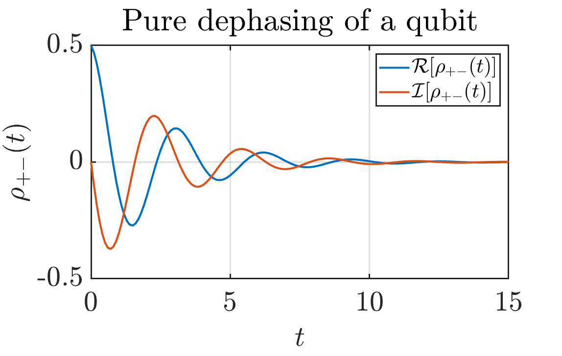
Pure dephasing
The Lindblad operator that gives rise to pure dephasing dynamics is given by <math-renderer class="js-inline-math" style="display: inline" data-static-url="https://github.githubassets.com/static" data-run-id="f8d2cf232f068143b380647b1c9d5574">$\sigma_z$</math-renderer>. Take a look the example file to see an instructive example on how to use the program in this case.

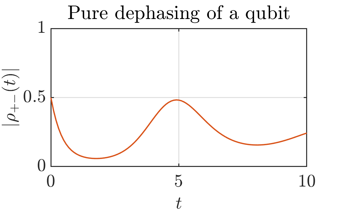
Time dependent pure dephasing
In this case a time dependent Hamiltonian and decay rate is given. The Lindblad operator is still <math-renderer class="js-inline-math" style="display: inline" data-static-url="https://github.githubassets.com/static" data-run-id="f8d2cf232f068143b380647b1c9d5574">$\sigma_z$</math-renderer> giving rise to pure dephasing. In this case the decay rate becomes negative at some intervals where the coherence experience revivals.

Cite As
Andreu Angles Castillo (2025). Lindblad-ME (https://github.com/dark-dryu/Lindblad-ME/releases/tag/v0.1), GitHub. Retrieved .
MATLAB Release Compatibility
Platform Compatibility
Windows macOS LinuxTags
Community Treasure Hunt
Find the treasures in MATLAB Central and discover how the community can help you!
Start Hunting!Discover Live Editor
Create scripts with code, output, and formatted text in a single executable document.
| Version | Published | Release Notes | |
|---|---|---|---|
| 0.1 |


