Physical Layer Abstraction for System-Level Simulation
This example demonstrates IEEE® 802.11ax™ physical layer abstraction for system-level simulation. A link quality model and link performance model based on the TGax evaluation methodology are presented and validated by comparing with published results.
Introduction
Modeling the full physical layer processing at each transmitter and receiver when simulating large networks is computationally expensive. Physical layer abstraction, or link-to-system mapping is a method to run simulations in a timely manner by accurately predicting the performance of a link in a computationally efficient way.
This example demonstrates physical layer abstraction for the data portion of an 802.11ax [ 1 ] packet based on the TGax evaluation methodology [ 2 ].
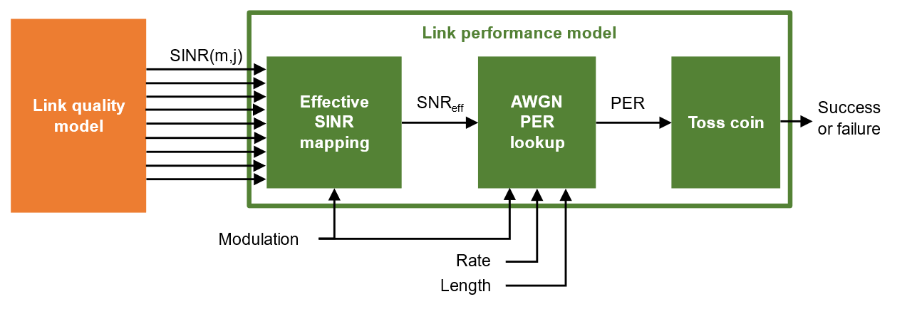
There are two parts to the physical layer abstraction model [ 3, 4 ]:
The link quality model calculates the post-equalizer signal to interference and noise ratio (SINR) per subcarrier. For a receiver, this is based on the location and transmission characteristics of the transmitter of interest, and interfering transmissions, and the impact of large- and small-scale fading.
The link performance model predicts the instantaneous packet error rate (PER), and therefore transmission success of an individual packet, given the SINR per subcarrier and coding parameters used for the transmission.

The example is split into two parts:
Part A demonstrates the link quality model used to obtain the SINR per subcarrier and validates it by comparing the results for a residential scenario as per the box 2 tests in the TGax evaluation methodology. The objective of box 2 tests is to align the distribution of small and large scale fading channels with MIMO configurations of TGax contributors.
Part B demonstrates the link performance model used to estimate the PER, and compares the result of using the abstraction against a link-level simulation with a fading TGax channel model as per the box 0 tests in the TGax evaluation methodology. The objective of box 0 tests is to align PHY abstractions of TGax contributors.
Part A - Link Quality Model
The link quality model implements the box 2 SINR equation from the TGax Evaluation Methodology. The multiple-input-multiple-output (MIMO) SINR per subcarrier (index ) and spatial stream (index ) between the transmitter and receiver of interest is given by
.
The SINR takes into account the path-loss and fading channels between all transmitters and the receiver, and precoding applied at the transmitters. The power of the signal of interest is given by
,
where is the received power of the signal of interest, is the linear receiver filter, is the channel matrix between the transmitter and receiver of interest, and is the precoding matrix applied at the transmitter.
The power of intra-user interference is given by
.
The power of inter-user interference is given by
,
where is the set of interfering transmitters in the th basic service set (BSS)
The noise power is given by
,
where is the noise power spectral density.
Generate a Channel Matrix per Subcarrier
The link quality model requires a channel matrix per subcarrier. Calculate the channel matrix from the path gains returned from the fading channel model wlanTGaxChannel by using the helperPerfectChannelEstimate function. Efficiently generate path gains by setting the ChannelFiltering property of wlanTGaxChannel to false.
sprev = rng('default'); % Seed random number generator and store previous state

% Get an HE OFDM configuration: 80 MHz channel bandwidth, 3.2 us guard
% interval
ofdmInfo = wlanHEOFDMInfo('HE-Data','CBW80',3.2);
k = ofdmInfo.ActiveFrequencyIndices;

% Configure channel to return path gains for one OFDM symbol
tgax = wlanTGaxChannel;
tgax.ChannelBandwidth = 'CBW80';
tgax.SampleRate = 80e6; % MHz
tgax.ChannelFiltering = false;
tgax.NumSamples = ofdmInfo.FFTLength+ofdmInfo.CPLength;

% Generate channel matrix per subcarrier for signal of interest
pathGains = tgax();    % Get path gains
chanInfo = info(tgax); % Get channel info for filter coefficients
chanFilter = chanInfo.ChannelFilterCoefficients;
Hsoi = helperPerfectChannelEstimate(pathGains,chanFilter,ofdmInfo);

% Generate channel matrix per subcarrier for interfering signal
reset(tgax); % Get a new channel realization
pathGains = tgax();
Hint = helperPerfectChannelEstimate(pathGains,chanFilter,ofdmInfo);
SINR Calculation
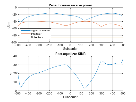
Calculate and visualize the post-equalizer SINR per subcarrier with the calculateSINR and plotSINR helper functions.
Psoi = -20; % Signal of interest received power (dBm)
Pint = -45; % Interfering signal received power (dBm)
N0 = -85;   % Noise power (dBm)
W = ones(ofdmInfo.NumTones,1); % Precoding matrix (assume no precoding)

sinr = calculateSINR(Hsoi,db2pow(Psoi-30),W,db2pow(N0-30),{Hint},db2pow(Pint-30),{W});

plotSINR(sinr,Hsoi,Psoi,Hint,Pint,N0,k);
TGax Evaluation Methodology Box 2 - Verify SINR Calibration
This section validates the SINR calculation by comparing the cumulative density function (CDF) of per-subcarrier SINRs with calibration results provided by the TGax working group. We compare the SINR calculation with results published by TGax [ 5 ] for box 2, test 3: "downlink transmission per basic channel access rule" for the residential scenario.
For more information about the scenario, and for the results of long-term SINR calibration see the 802.11ax PHY-Focused System-Level Simulation example.
The major simulation parameters are defined as either belonging to Physical Layer (PHY), Medium Access Control Layer (MAC), scenario, or simulation. In this example the PHY and MAC parameters are assumed to be the same for all nodes.
sinrCalibration =true; % Disable box 2 calibration if sinrCalibration PHYParams = struct; PHYParams.TxPower = 20; % Transmitter power in dBm PHYParams.TxGain = 0; % Transmitter antenna gain in dBi PHYParams.RxGain = -2; % Receiver antenna gain in dBi PHYParams.NoiseFigure = 7; % Receiver noise figure in dB PHYParams.NumTxAntennas = 1; % Number of transmitter antennas PHYParams.NumSTS = 1; % Number of space-time streams PHYParams.NumRxAntennas = 1; % Number of receiver antennas PHYParams.ChannelBandwidth = 'CBW80'; % Bandwidth of system PHYParams.TransmitterFrequency = 5e9; % Transmitter frequency in Hz MACParams = struct; MACParams.NumChannels = 3; % Number of non-overlapping channels MACParams.CCALevel = -70; % Transmission threshold in clear channel assessment algorithm (dBm)
The scenario parameters define the size and layout of the residential building as per [ 6 ]. Note only one receiver (STA) can be active at any given time.
ScenarioParams = struct;
ScenarioParams.BuildingLayout = [10 2 5]; % Number of rooms in [x,y,z] directions
ScenarioParams.RoomSize = [10 10 3];      % Size of each room in meters [x,y,z]
ScenarioParams.NumRxPerRoom = 1;          % Number of receivers per room.
The NumDrops and NumTxEventsPerDrop parameters control the length of the simulation. In this example, these parameters are configured for a short simulation. A 'drop' randomly places transmitters and receivers within the scenario and selects the channel for a BSS. A 'transmission' event randomly selects transmitters and receivers for transmissions according to the basic clear channel assessment (CCA) rules defined in the evaluation methodology.
SimParams = struct;
SimParams.Test = 3; % Downlink transmission per basic channel access rule
SimParams.NumDrops = 3;
SimParams.NumTxEventsPerDrop = 2;
The function box2Simulation runs the simulation by performing these steps:
Randomly drop transmitters (APs) and receivers (STAs) within the scenario.
Calculate the large-scale path loss and generate frequency-selective TGax fading channels for all non-negligible links.
For each transmission event, determine active transmitters and receivers based on CCA rules.
Calculate and return the SINR per subcarrier and the effective SINR for each active receiver as per box 2, test 3 in the TGax evaluation methodology.
box2Results = box2Simulation(PHYParams,MACParams,ScenarioParams,SimParams);
Plot the CDF of the SINR per subcarrier and effective SINR (as defined in box 2, test 3) against submitted calibration results.
tgaxCalibrationCDF(box2Results.sinr(:), ...
    ['SS1Box2Test' num2str(SimParams.Test) 'A'],'CDF of SINR per subcarrier');
tgaxCalibrationCDF(box2Results.sinrEff(:), ...
    ['SS1Box2Test' num2str(SimParams.Test) 'B'],'CDF of effective SINR per reception');

end
  Running drop #1/3 ...
    Generating 3518 fading channel realizations ...
    Running transmission event #1/2 ...
    Running transmission event #2/2 ...
  Running drop #2/3 ...
    Generating 3366 fading channel realizations ...
    Running transmission event #1/2 ...
    Running transmission event #2/2 ...
  Running drop #3/3 ...
    Generating 3750 fading channel realizations ...
    Running transmission event #1/2 ...
    Running transmission event #2/2 ...
![Figure contains an axes object. The axes object with title Calibration: CDF of SINR per subcarrier, xlabel SINR [dB], ylabel CDF contains 11 objects of type line. These objects represent Calibrated Curves, WLAN Toolbox.](../../examples/wlan/win64/PHYAbstractionExample_03.png)
![Figure contains an axes object. The axes object with title Calibration: CDF of effective SINR per reception, xlabel SINR [dB], ylabel CDF contains 12 objects of type line. These objects represent Calibrated Curves, WLAN Toolbox.](../../examples/wlan/win64/PHYAbstractionExample_04.png)
Increase the number of drops for a more accurate comparison.
Part B - Link Performance Model
The link performance model predicts the instantaneous PER given the SINR per subcarrier calculated in Part A and coding parameters used for the transmission.
Effective SINR mapping and averaging is used to compress the post-equalizer SINR per subcarrier into a single effective SNR. The effective SNR is the SNR that provides an equivalent PER performance with an additive white Gaussian noise (AWGN) channel as with the fading channel. A pre-computed lookup table, generated with WLAN Toolbox™, provides the PER for an SNR under an AWGN channel for a given channel coding, modulation scheme, and coding rate. Once the PER is obtained, a random variable determines whether the packet has been received in error.
The TGax evaluation methodology PER estimation procedure is used in this example considering a single interference event.
The effective SINR is calculated using the received bit mutual information rate (RBIR) mapping function;
.
is the RBIR mapping function, which transforms the SINR of each subcarrier to an “information measure" for the modulation scheme . The RBIR mapping function for BPSK, QPSK, 16QAM, 64QAM and 256QAM is provided in [ 7 ].
is the inverse RBIR mapping function, which transforms an “information measure” back to the SNR domain.
is the number of spatial-streams.
is the number of subcarriers.
is the post-equalizer SINR of the th subcarrier and th spatial-stream.
and are tuning parameters. The TGax evaluation methodology assumes no tuning therefore in this example we assume these are set to 1.
The PER for a reference data length is obtained by looking up the appropriate AWGN table, , given the modulation and coding scheme (MCS), channel coding scheme, and reference data length ()
,
where the reference data length depends on the channel coding and data length for the transmission .
.
The final estimated PER is then adjusted for the data length:
.
The described method assumes the SINR is constant for the duration of the packet. The TGax evaluation methodology describes techniques to deal with time-varying interference and estimate the error rate of media access control protocol data units (MPDUs) within an aggregate MPDU (A-MPDU).
Calculate Effective SINR
Calculate the effective SINR and the PER using the tgaxLinkPerformanceModel example helper object. The effectiveSINR method calculates the effective SINR given the modulation scheme and post equalizer SINR per subcarrier and spatial stream.
format ='HE_SU'; mcs =
6; % MCS 6 is 64-QAM [snreff,rbir_sc,rbir_av] = tgaxLinkPerformanceModel.effectiveSINR(sinr,format,mcs);
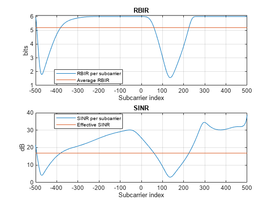
The RBIR (information measure) per subcarrier obtained by mapping the SINR per subcarrier, and the average RBIR are shown in the first figure subplot. The effective SINR per subcarrier is obtained by inverse mapping the average RBIR and is shown in the second subplot.
plotRBIR(sinr,snreff,rbir_av,rbir_sc,k);
Estimate Packet Error Rate
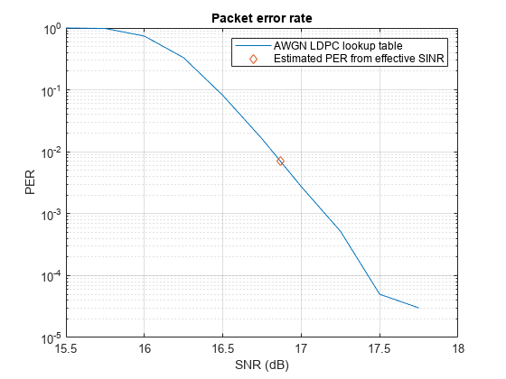
Given the effective SNR, estimate the PER by linearly interpolating and extrapolating a pre-computed AWGN link-level curve in the logarithmic domain, and adjusting for the data length. The estimatePER method returns the final PER, per, and the AWGN lookup table used, lut .
channelCoding ="LDPC"; dataLength =
1458; % Bytes [per,~,~,lut] = tgaxLinkPerformanceModel.estimatePER(snreff,format,mcs,channelCoding,dataLength); % Plot the AWGN lookup table and the estimated PER figure; semilogy(lut(:,1),lut(:,2)); grid on hold on plot(snreff,per,'d'); legend('AWGN LDPC lookup table','Estimated PER from effective SINR') title('Packet error rate') xlabel('SNR (dB)') ylabel('PER')
TGax Evaluation Methodology Box 0 - Verify Effective SNR vs PER Performance
To verify the entire physical-layer abstraction method, the PER from a link-level simulation is compared with the PER estimates using the abstraction. This follows steps 2 and 3 of box 0 testing in the TGax Evaluation Methodology. An 802.11ax single-user link is modeled with perfect synchronization, channel estimation, and no impairments apart from a fading TGax channel model and AWGN. Only errors within data portion of a packet are considered.
In this example the SNRs to simulate are selected based on the MCS, number of transmit and receive antennas, and channel model for the given PHY configuration. The number of space-time streams is assumed to equal the number of transmit antennas. The simulation is configured for a short run; for more meaningful results you should increase the number of packets to simulate.
verifyAbstraction =true; % Disable box 0 simulation if verifyAbstraction % Simulation Parameters mcs = [4 8]; % Vector of MCS to simulate between 0 and 11 numTxRx = [1 1]; % Matrix of MIMO schemes, each row is [numTx numRx] chan = "Model-D"; % String array of delay profiles to simulate maxNumErrors = 1e1; % The maximum number of packet errors at an SNR point maxNumPackets = 1e2; % The maximum number of packets at an SNR point % Fixed PHY configuration for all simulations cfgHE = wlanHESUConfig; cfgHE.ChannelBandwidth = 'CBW20'; % Channel bandwidth cfgHE.APEPLength = 1000; % Payload length in bytes cfgHE.ChannelCoding = 'LDPC'; % Channel coding % Generate a structure array of simulation configurations. Each element is % one SNR point to simulate. simParams = getBox0SimParams(chan,numTxRx,mcs,cfgHE,maxNumErrors,maxNumPackets); % Simulate each configuration results = cell(1,numel(simParams)); % parfor isim = 1:numel(simParams) % Use 'parfor' to speed up the simulation for isim = 1:numel(simParams) results{isim} = box0Simulation(simParams(isim)); end
The suitability of the abstraction is determined by comparing the PER calculated by link-level simulation and abstraction. The first figure compares the PERs at each SNR simulated.
plotPERvsSNR(simParams,results);
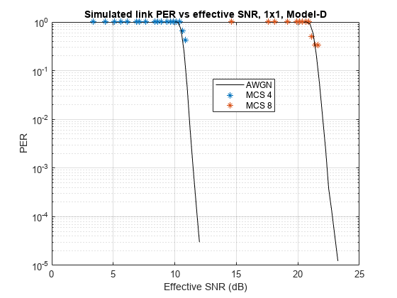
The second figure compares the number of successfully decoded link-level simulation packets with an effective SNR against the reference AWGN curve. If the abstraction is successful the PER should follow the AWGN curve.
plotPERvsEffectiveSNR(simParams,results);
end
Model-D 1-by-1, MCS 4, SNR 11 completed after 14 packets, PER:0.78571 Model-D 1-by-1, MCS 4, SNR 15 completed after 22 packets, PER:0.5 Model-D 1-by-1, MCS 4, SNR 19 completed after 100 packets, PER:0.05 Model-D 1-by-1, MCS 4, SNR 23 completed after 100 packets, PER:0.02 Model-D 1-by-1, MCS 4, SNR 27 completed after 100 packets, PER:0 Model-D 1-by-1, MCS 8, SNR 21.5 completed after 13 packets, PER:0.84615 Model-D 1-by-1, MCS 8, SNR 25.5 completed after 23 packets, PER:0.47826 Model-D 1-by-1, MCS 8, SNR 29.5 completed after 100 packets, PER:0.03 Model-D 1-by-1, MCS 8, SNR 33.5 completed after 100 packets, PER:0.02 Model-D 1-by-1, MCS 8, SNR 37.5 completed after 100 packets, PER:0

rng(sprev) % Restore random stateIn this example the tuning parameters and are set to 1. These could be tuned to further improve the accuracy of the abstraction if desired. The results when simulating 1000 packet errors or 100000 packets for MCS 0 to 9 for a 1458-byte packet without tuning is shown.


Selected Bibliography
IEEE Std 802.11™-2024 IEEE Standard for Information technology - Telecommunications and information exchange between systems - Local and metropolitan area networks - Specific requirements - Part 11: Wireless LAN Medium Access Control (MAC) and Physical Layer (PHY) Specifications.
IEEE 802.11-14/0571r12 - 11ax Evaluation Methodology.
Brueninghaus, Karsten, et al. "Link performance models for system level simulations of broadband radio access systems." 2005 IEEE 16th International Symposium on Personal, Indoor and Mobile Radio Communications. Vol. 4. IEEE, 2005.
Mehlführer, Christian, et al. "The Vienna LTE simulators-Enabling reproducibility in wireless communications research." EURASIP Journal on Advances in Signal Processing 2011.1 (2011): 29.
IEEE 802.11-14/0800r30 - Box 1 and Box 2 Calibration Results.
IEEE 802.11-14/0980r16 - TGax Simulation Scenarios.
IEEE 802.11-14/1450r0 - Box 0 Calibration Results