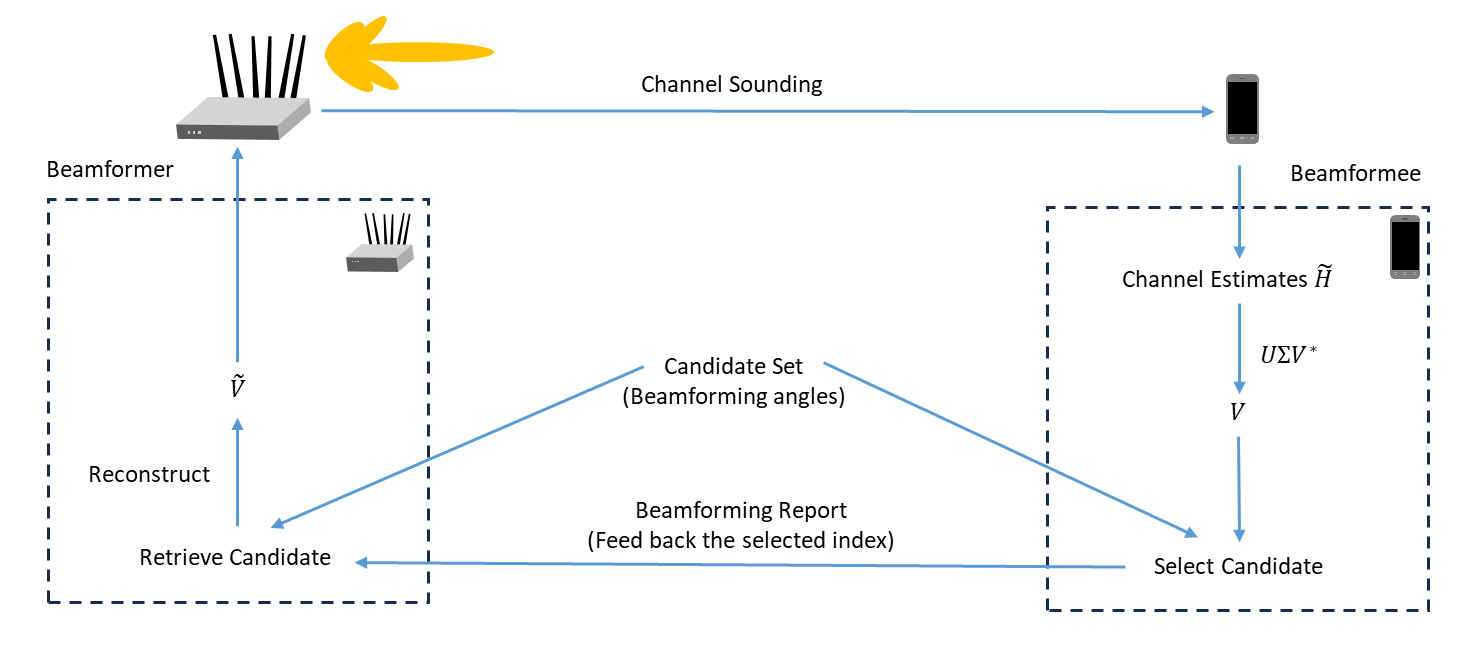
CSI Feedback Compression for 802.11be Using AI

Since R2025a

This example shows how to compress channel state information (CSI) in an IEEE® 802.11be™ (Wi-Fi® 7) SU-MIMO beamforming scenario. To enhance CSI feedback compression, it uses a k-means-based AI technique.

Introduction

In 802.11 networks, CSI feedback compression techniques are crucial for efficient wireless communication. These techniques reduce the overhead of transmitting CSI from the beamformee back to the beamformer. For example, the 802.11ax and 802.11be standards define a series of quantization resolutions that compress the CSI for SU-MIMO and MU-MIMO scenarios in the form of angles [1] [2]. (For details, see 802.11ax Compressed Beamforming Packet Error Rate Simulation). Despite achieving acceptable compression through standardized quantization methods, large amounts of overhead or prolonged sounding procedures can negatively affect the latency and limit system performance for large numbers of transmit antennas and space-time streams. As a result, the communication between stations (STAs) and multiple access points (APs) that perform joint or coordinated transmissions requires further reduction of CSI feedback overhead [3].

For CSI compression, this example implements the iFOR algorithm [4], which is based on the k-means unsupervised learning approach, to classify angle vectors derived from the beamforming matrix, which is commonly referred to as the V matrix. In the iFOR algorithm, the compressed feedback from a STA (beamformee) to an AP (beamformer) is generated by using a fixed number of candidate vectors to minimize and control the number of bits required to feed back the CSI. In the training phase, the example runs a simulation to generate a large empirical data set. It then feeds this data into a k-means clustering algorithm. Through the selection of an appropriate value of k, the centroids of these clusters can serve as the candidate set, with this information assumed to be shared between the beamformee and the beamformer. During the deployment, the beamformee calculates the CSI feedback vector and then finds the candidate vector with the lowest Euclidean distance.

Configure 802.11be Waveform

You can configure the transmission and channel model for customized training and testing. This example configures an 802.11be SU-MIMO transmission scenario using four transmit antennas and two space-time streams.

simParams = struct;
simParams.ChannelBandwidth = 'CBW20';
simParams.NumTransmitAntennas = 4;
simParams.NumSpaceTimeStreams = 2;
simParams.APEPLength = 1e3;

Configure CSI Feedback Compression

This example does not model subcarrier beamforming smoothing. To sound all subcarriers and estimate the channel without interpolation for this transmission configuration, use the combination of 4x EHT-LTF compression mode and guard interval of 3.2 μs for transmission. To reduce the CSI feedback overhead, you can group the four subcarriers.

simParams.NumBitsPhi = 6; % Number of bits for phi for 802.11be baseline
simParams.NumBitsPsi = 4; % Number of bits for psi for 802.11be baseline
simParams.Ng = 4;         % Subcarrier grouping

Configure Channel

Configure the channel model between the beamformer and beamformee. See wlanTGaxChannel for details.

simParams.Channel = wlanTGaxChannel;
simParams.Channel.DelayProfile = 'Model-D';
simParams.Channel.NumTransmitAntennas = simParams.NumTransmitAntennas;
simParams.Channel.NumReceiveAntennas = simParams.NumSpaceTimeStreams; % Same as that of spatial time streams
simParams.Channel.TransmitReceiveDistance = 5; % Distance in meters
simParams.Channel.ChannelBandwidth = simParams.ChannelBandwidth;
simParams.Channel.LargeScaleFadingEffect = 'None';
simParams.Channel.NormalizeChannelOutputs = false;
simParams.Channel.SampleRate = wlanSampleRate(simParams.ChannelBandwidth);

Train AI Model for CSI Feedback Compression

You can train the k-means model by simulating the CSI feedback compression scenario. You can also specify the number of packets and the signal-to-noise ratio (SNR) range for generating the training data. This example simulates the link between a beamformer and a beamformee, using different channel realizations for multiple packets to obtain the CSI feedback vector. The k-means model uses 10 bits to create a codebook of size 1024 for CSI feedback compression. This codebook size can significantly reduce the feedback overhead while maintaining an acceptable loss in the accuracy of the CSI feedback [4]. This example sets the maximum number of iterations for k-means training as 100. You can increase this number if the result of k-means does not converge. When the training is complete, this example generates the trained model.

For simplicity, this example uses a small data set, which results in a short simulation time. For more accurate results, use a larger data set. The example provides the pretrained model to show the high levels of performance that can be achieved with more training data. The pretrained model was trained for with an SNR range of 0 dB to 40 dB with a step of 2 dB, 1000 packets per SNR point and maximum number of iterations of 1000. Other configurations are same as example default. This example trains the model in real-time by default, but you can set simParams.UsePreTrainedModel to true to use the aforementioned pretrained model.

simParams.NumPackets = 1e2;
simParams.SNRRange = 8.5:2:14.5;
simParams.NumBitsAICompression = 10;
simParams.NumMaxInterations = 1e2;
simParams.UsePreTrainedModel = false;
if ~simParams.UsePreTrainedModel
    trainedModel = trainCSIFeedbackCompression(simParams);
else
    load("trainedModel_CSIFeedbackCompression.mat")
end

Training is finished and the trained model is ready for testing.

Test AI Model for CSI Feedback Compression

Evaluate the performance of the trained k-means model you obtained from the training phase. You can specify the modulation and coding scheme (MCS) range for the performance evaluation. This example uses different seeds for training and testing to ensure randomness between training and testing data.

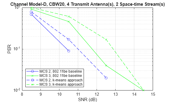
During the testing phase, this example simulates the CSI feedback compression approach (phi = 6, psi = 4 as specified in Table 9-55 of [1]). This example uses this approach as the performance baseline. The packet error rate (PER) performance of both the 802.11be baseline and the k-means approaches is showcased at the end of the testing phase. For the same MCS, the PER degrades between 1 dB and 2 dB from the iFOR algorithm to the baseline. This degradation is expected because the number of bits in the CSI feedback has vastly reduced in the iFOR method.

simParams.TrainedModel = trainedModel;
simParams.MCSRange = [2,3];
% PER simulation for 802.11be baseline (NumBitsPhi = 6 and NumBitsPsi = 4 and) vs k-means approach
packetErrorRatePerMCSPerSNR = testCSIFeedbackCompression(simParams); % PER is size NumMCS-by-NumSNR-by-2

802.11be baseline simulation: MCS 2, SNR 8.5 dB completed after 16 packets, PER:0.6875
802.11be baseline simulation: MCS 2, SNR 10.5 dB completed after 100 packets, PER:0.09
802.11be baseline simulation: MCS 2, SNR 12.5 dB completed after 100 packets, PER:0
802.11be baseline simulation: MCS 2, SNR 14.5 dB completed after 100 packets, PER:0


802.11be baseline simulation: MCS 3, SNR 8.5 dB completed after 12 packets, PER:0.91667
802.11be baseline simulation: MCS 3, SNR 10.5 dB completed after 24 packets, PER:0.45833
802.11be baseline simulation: MCS 3, SNR 12.5 dB completed after 100 packets, PER:0.04
802.11be baseline simulation: MCS 3, SNR 14.5 dB completed after 100 packets, PER:0.01


IFOR algorithm simulation: MCS 2, SNR 8.5 dB completed after 14 packets, PER:0.78571
IFOR algorithm simulation: MCS 2, SNR 10.5 dB completed after 65 packets, PER:0.16923
IFOR algorithm simulation: MCS 2, SNR 12.5 dB completed after 100 packets, PER:0.02
IFOR algorithm simulation: MCS 2, SNR 14.5 dB completed after 100 packets, PER:0


IFOR algorithm simulation: MCS 3, SNR 8.5 dB completed after 11 packets, PER:1
IFOR algorithm simulation: MCS 3, SNR 10.5 dB completed after 18 packets, PER:0.61111
IFOR algorithm simulation: MCS 3, SNR 12.5 dB completed after 65 packets, PER:0.16923
IFOR algorithm simulation: MCS 3, SNR 14.5 dB completed after 100 packets, PER:0.01

Choose MCS and Compare Goodput

Goodput refers to the effective amount of useful data transmitted over a network within a specific time period. It measures the data that successfully arrives at its intended destination and is usable by the recipient. It provides a more realistic assessment of network performance by emphasizing the data that is pertinent to the end user. The link-level goodput is defined as:

$$\mathrm{goodput}=\frac{\mathrm{L}\left(1-\mathrm{PER}\right)}{{\mathit{T}}_{\mathrm{sounding}}+{\mathit{T}}_{\mathrm{data}}+{\mathit{T}}_{\mathrm{ACK}}}$$

where $\mathrm{L}$ is the length of the payload in bits, ${\mathit{T}}_{\mathrm{sounding}}$is the total time duration for the channel sounding protocol, ${\mathit{T}}_{\mathrm{data}}$ is the time duration for data transmission, and ${\mathit{T}}_{\mathrm{ACK}}$ is the time duration of the ACK transmission.

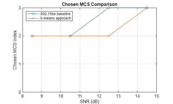
To calculate the goodput, determine the PER of a chosen MCS at a given SNR. The chosen MCS is the highest MCS index that remains below a predefined PER threshold, known as the target PER. This example first plots the chosen MCS for each SNR of both the 802.11be baseline and the k-means approach, with a target PER of 0.1. At a SNR of 12.5 dB, the 802.11be baseline approach chooses MCS 3 as the PER, which is below 0.1 according to the PER plot above, while the k-means approach chooses MCS 2 since the PER does not meet the target requirement.

targetPER = 0.1;
chosenMCS = chooseMCS(simParams,packetErrorRatePerMCSPerSNR,targetPER);

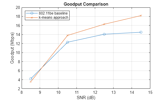
Using the chosen MCS above, you can calculate the goodput. This example uses MCS 2 to feed back the beamforming frame. (For details about the time-related values, see Table 1 of [4]). The goodput comparison plot shows that, compared to the 802.11be baseline approach, the iFOR algorithm offers a substantial improvement in goodput despite the slight degradation of PER performance. This improvement is due to the significant reduction in the number of CSI feedback bits, which dramatically shortens the duration of the sounding protocol.

goodput = calculateGoodput(simParams,packetErrorRatePerMCSPerSNR,chosenMCS);

Further Exploration

The cfgSim.NumPackets parameter controls the number of packets simulated for each SNR point. Increase this value for meaningful results. Furthermore, the range of SNR and MCS affects the performance of the trained k-means model. Expand the range of SNR and MCS lead to see more meaningful results of chosen MCS and goodput.

References

[1] IEEE Draft Standard for Information Technology–Telecommunications and Information Exchange between Systems Local and Metropolitan Area Networks–Specific Requirements - Part 11: Wireless LAN Medium Access Control (MAC) and Physical Layer (PHY) Specifications Amendment: Enhancements for Extremely High Throughput (EHT)." IEEE P802.11be/D7.0, August 2024.

[2] IEEE Std 802.11ax™-2021. IEEE Standard for Information Technology - Telecommunications and Information Exchange between Systems - Local and Metropolitan Area Networks - Specific Requirements - Part 11: Wireless LAN Medium Access Control (MAC) and Physical Layer (PHY) Specifications - Amendment 1: Enhancements for High-Efficiency WLAN.

[3] IEEE 802.11 AIML TIG Technical Report Draft, IEEE 802.11-22/0987r25, 2024.

[4] M.Deshmukh. et al. Intelligent Feedback Overhead Reduction (iFOR) in Wi-Fi 7 and Beyond, in Proceedings of 2022 VTC-Spring