Wavelet Time Scattering Classification of Phonocardiogram Data

Data Description

This example uses phonocardiogram (PCG) data obtained from persons with normal and abnormal cardiac function. The dataset consists of 3829 recordings, 2575 from persons with normal cardiac function and 1254 records from persons with abnormal cardiac function. Each recording is 10,000 samples long and is sampled at 2 kHz. This represents five seconds of phonocardiogram data. The dataset is constructed from the training and validation data used in the PhysioNet Computing in Cardiology Challenge 2016 [1][2].

Download Data

The first step is to download the data from the GitHub repository. To download the data, click Code and select Download ZIP. Save the file physionet_phonocardiogram-main.zip in a folder where you have write permission. The instructions for this example assume you have downloaded the file to your temporary directory, (tempdir in MATLAB®). Modify the subsequent instructions for unzipping and loading the data if you choose to download the data in folder different from tempdir.

The file physionet_phonocardiogram-main.zip contains

and PCG_Data.zip contains

heartSoundData.mat holds the data and class labels used in this example. The .txt file, Modified_physionet_data.txt, is required by PhysioNet's copying policy and provides the source attributions for the data as well as a description of how each signal in heartSoundData.mat corresponds to a file in the original PhysioNet data. extrafiles.mat also contains source file attributions and is explained in the Modified_physionet_data.txt file. The only file required to run the example is heartSoundData.mat.

Load Data

If you followed the download instructions in the previous section, enter the following commands to unzip the two archive files.

unzip(fullfile(tempdir,"physionet_phonocardiogram-main.zip"),tempdir)
unzip(fullfile(tempdir,"physionet_phonocardiogram-main","PCG_Data.zip"), ...
    fullfile(tempdir,"PCG_Data"))

After you unzip the PCG_Data.zip file, load the data into MATLAB.

load(fullfile(tempdir,"PCG_Data","heartSoundData.mat"))

heartSoundData is a structure array with two fields: Data and Classes. Data is a 10000-by-3829 matrix where each column is an PCG recording. Classes is a 3829-by-1 categorical array of diagnostic labels, one for each column of Data. Because this is a binary classification problem, the classes are "normal" and "abnormal". As previously stated, there are 2575 normal records and 1254 abnormal records. Equivalently, 67.25% of the examples in the data are from persons with normal cardiac function while 32.75% are from persons with abnormal cardiac function. You can verify this by entering:

countlabels(heartSoundData.Classes)

ans = 2×3 table
      normal    2575    67.2499
    abnormal    1254    32.7501

Wavelet Scattering Network

Use waveletScattering to construct a wavelet time scattering network. Set the invariant scale to match the signal length. The default scattering network has two wavelet transforms (filter banks). The first wavelet filter bank has eight wavelets per octave. The second filter bank has one wavelet per octave. Set the 'OptimizePath' property to true.

N = 1e4;
sn = waveletScattering(SignalLength=N,InvarianceScale=N, ...
    OptimizePath=true);

Create Training and Test Sets

Split the data into a training and test set. Allocate 70% of the data for training and the remaining 30% for test.

rng default;
idxTrainTest = splitlabels(heartSoundData.Classes,0.7);
trainData = heartSoundData.Data(:,idxTrainTest{1});
testData = heartSoundData.Data(:,idxTrainTest{2});
trainLabels = heartSoundData.Classes(idxTrainTest{1});
testLabels = heartSoundData.Classes(idxTrainTest{2});

You can check the count and percentage of each class in the training and test sets to confirm that splitlabels has performed a stratified random sampling of the data.

countlabels(trainLabels)

ans = 2×3 table
      normal    1802    67.2388
    abnormal     878    32.7612

countlabels(testLabels)

ans = 2×3 table
      normal    773    67.2759
    abnormal    376    32.7241

Scattering Features

Obtain the scattering transform of all 2680 recordings in the training set. For multivariate time series, the scattering transform assumes each column is a separate signal. Use the "log" option to obtain the natural logarithm of the scattering coefficients.

scat_features_train = featureMatrix(sn,trainData,Transform="log");

For the given scattering parameters, scat_features_train is a 279-by-5-by-2680 matrix. There are 279 scattering paths and five scattering windows for each of the 2680 signals. In order to pass this to the SVM classifier, reshape the tensor into a 13400-by-279 matrix where each row represents a single scattering window across the 279 scattering paths. The total number of rows is equal to the product of 5 and 2680 (number of recordings in the training data).

Nseq = size(scat_features_train,2);
scat_features_train = permute(scat_features_train,[2 3 1]);
scat_features_train = reshape(scat_features_train, ...
    size(scat_features_train,1)*size(scat_features_train,2),[]);

Repeat the process for the test data.

scat_features_test = featureMatrix(sn,testData,Transform="log");
scat_features_test = permute(scat_features_test,[2 3 1]);
scat_features_test = reshape(scat_features_test, ...
    size(scat_features_test,1)*size(scat_features_test,2),[]);

Here we replicate the labels so that we have a label for each scattering time window.

[sequence_labels_train,sequence_labels_test] = ...
    createSequenceLabels_heartsounds(Nseq,trainLabels,testLabels);

Fit the SVM to the training data. In this example, we use a cubic polynomial kernel. After fitting the SVM to the training data, we perform a 5-fold cross-validation to estimate the generalization error on the training data. Here each scattering window is classified separately.

Because the data is highly imbalanced, specify a misclassification cost matrix. The ratio of normal phonocardiograms to abnormal ones is approximately 2:1. In other words, approximately 2/3 of the data are normal phonocardiograms and 1/3 are abnormal. Accordingly, specify the misclassification matrix as $$\left(\begin{array}{cc}0& 2\\ 1& 0\end{array}\right)$$ with ClassNames = ["abnormal" "normal"].The given penalty structure deliberately trades normal-class recall for abnormal-class recall. In applications like medical screening, this is usually the right trade-off because it is typically better to have false positives than to miss genuine abnormalities. This does mean however, that recall for the abnormal class will likely be significantly higher than precision. You can always balance this for the cost considerations of your application by changing the values in the Cost matrix.

classNames = categorical(["abnormal" "normal"]);
classificationSVM = fitcsvm( ...
    scat_features_train, ...
    sequence_labels_train , ...
    KernelFunction="polynomial", ...
    PolynomialOrder=3, ...
    KernelScale="auto", ...
    BoxConstraint=1, ...
    Standardize=true, ...
    ClassNames=classNames,...
    Cost=[0 2; 1 0]);
kfoldmodel = crossval(classificationSVM, KFold=5);

Compute the cross-validation loss as a percentage and display the confusion matrix.

predLabels = kfoldPredict(kfoldmodel);
loss = kfoldLoss(kfoldmodel)*100;
fprintf("Loss is %2.2f percent\n",loss);

Loss is 1.03 percent

accuracy = 100-loss;
fprintf("Accuracy is %2.2f percent\n",accuracy);

Accuracy is 98.97 percent

confmatCV = confusionchart(sequence_labels_train,predLabels, ...
ColumnSummary="column-normalized",RowSummary="row-normalized");

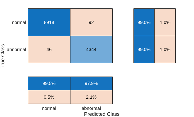
Note that the scattering network results in approximately 99 percent accuracy when each time window is classified separately. However, the performance is actually better than this value because we have five scattering windows per recording and the 99 percent accuracy is based on classifying all windows separately. In this case, use a majority vote to obtain a single class assignment per recording. The class vote corresponds to the mode of the votes for the scattering windows. If no unique mode is found, the helper function helperMajorityVote classifies that set of scattering windows as "NoUniqueMode" to indicate a classification error. This results in an extra column in the confusion matrix. Note in this case, an assignment of "NoUniqueMode" is not possible because there are an odd number of votes and it is a binary classification problem. The possibility of a non-unique mode is included for completeness in case you wish to modify the example in a manner which results in an even number of votes.

ClassVotes = helperMajorityVote(predLabels,trainLabels,classNames);
CVaccuracy = sum(eq(ClassVotes,trainLabels))./numel(trainLabels)*100;
fprintf("The true cross-validation accuracy is %2.2f percent.\n",CVaccuracy);

The true cross-validation accuracy is 99.63 percent.

Display the confusion matrix for the majority vote classifications.

cmCV = confusionchart(trainLabels,ClassVotes, ...
ColumnSummary="column-normalized",RowSummary="row-normalized");
title("Cross-Validation Accuracy -- Majority Vote")

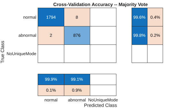
The cross-validation accuracy on the training data is actually higher than 99 percent. There are 8 normal records, which are classified as abnormal. Two abnormal records are classified as normal.

Use the trained SVM model to make class predictions on the held-out test data.

predTestLabels = predict(classificationSVM,scat_features_test);

Determine the accuracy of the predictions on the test set using a majority vote.

ClassVotes = helperMajorityVote(predTestLabels,testLabels,classNames);
testaccuracy = sum(eq(ClassVotes,testLabels))./numel(testLabels)*100;
fprintf("The test accuracy is %2.2f percent.\n",testaccuracy);

The test accuracy is 92.08 percent.

Plot the confusion matrix.

cmTest = confusionchart(testLabels,ClassVotes, ...
ColumnSummary="column-normalized", ...
RowSummary="row-normalized");
title("Wavelet Scattering with SVM -- Majority Vote")

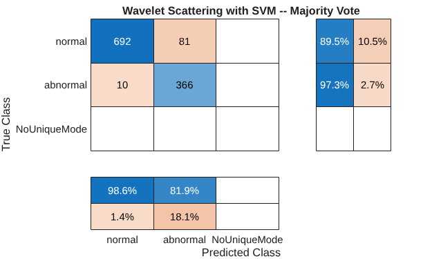
Of the 1149 test records, approximately 92% are correctly classified as "Normal" or "Abnormal". Of the 773 normal PCG recordings in the test set, 692 are correctly classified. Of the 376 abnormal recordings in the test set, 366 are correctly classified.

Compute the F1 scores and display the macro-averaged precision, recall, and F1 scores using the helperF1heartSounds helper function.

PRTable = helperF1heartSounds(cmTest.NormalizedValues);
disp(PRTable)

                     Precision    Recall    F1_Score
                     _________    ______    ________

    Abnormal          81.879       97.34     88.943 
    Normal            98.575      89.521     93.831 
    Macro Average     90.227      93.431     91.387 

Summary

This example used wavelet time scattering to robustly identify human phonocardiogram recordings as normal or abnormal in a binary classification problem. Wavelet scattering required only the specification of a single parameter, the length of the scale invariant, in order to produce low-variance representations of the PCG data that enabled the support vector machine classifier to accurately model the difference between the two groups. The support vector machine classifier with wavelet scattering was able to achieve superior performance in both precision and recall for both groups in spite of significantly unbalanced numbers of normal and abnormal PCG recordings in both the training and test set.

References

Supporting Functions

createSequenceLabels_heartsounds creates class labels for the wavelet time scattering sequences.

function [sequence_labels_train,sequence_labels_test] = createSequenceLabels_heartsounds(Nseq,trainLabels,testLabels)
% This function is only in support of the Wavelet Time Scattering 
% Classification of Phonocardiogram Data example. It may change or be
% removed in a future release.
Ntrain = numel(trainLabels);
trainLabels = repmat(trainLabels',Nseq,1);
sequence_labels_train = reshape(trainLabels,Nseq*Ntrain,1);
Ntest = numel(testLabels);
testLabels = repmat(testLabels',Nseq,1);
sequence_labels_test = reshape(testLabels,Ntest*Nseq,1);
end

helperMajorityVote implements a majority vote for a classification based on the mode. If no unique mode is present, a vote of NoUniqueMode is returned to ensure a classification error is recorded.

function [ClassVotes,ClassCounts] = helperMajorityVote(predLabels,origLabels,classes)
% This function is in support of Wavelet Toolbox examples. It may
% change or be removed in a future release.
% Make categorical arrays if the labels are not already categorical
predLabels = categorical(predLabels);
origLabels = categorical(origLabels);
% Expects both predLabels and origLabels to be categorical vectors
Npred = numel(predLabels);
Norig = numel(origLabels);
Nwin = Npred/Norig;
predLabels = reshape(predLabels,Nwin,Norig);
assert(size(predLabels,2) == length(origLabels));
ClassCounts = countcats(predLabels);
[~,idx] = max(ClassCounts);
ClassVotes = classes(idx);
% Check for any ties in the maximum values and ensure they are marked as
% error if the mode occurs more than once
modecnt = modecount(predLabels,string(classes));
ClassVotes(modecnt>1) = categorical("NoUniqueMode");
ClassVotes = ClassVotes(:);
%-------------------------------------------------------------------------
function modecnt = modecount(predlabels,classes)
% Ensure there is a unique mode
modecnt = zeros(size(predlabels,2),1);
for nc = 1:size(predlabels,2)
    hc = histcounts(predlabels(:,nc),classes);
    hc = hc-max(hc);
    if sum(hc == 0) > 1
        modecnt(nc) = 1;
    end
end
end
end

helperF1heartSounds calculate precision, recall, and F1 scores for the classifier results.

function PRTable = helperF1heartSounds(confmat)
% This function is only in support of the Wavelet Time Scattering 
% Classification of Phonocardiogram Data example. It may change or be
% removed in a future release.
precisionAB = confmat(2,2)/sum(confmat(:,2))*100;
precisionNR = confmat(1,1)/sum(confmat(:,1))*100 ;
recallAB = confmat(2,2)/sum(confmat(2,:))*100;
recallNR = confmat(1,1)/sum(confmat(1,:))*100;
F1AB = 2*(precisionAB*recallAB)/(precisionAB+recallAB);
F1NR = 2*(precisionNR*recallNR)/(precisionNR+recallNR);
MacroAverages = mean(cat(2,[precisionAB; precisionNR],...
    [recallAB;recallNR], [F1AB;F1NR]));
% Construct a MATLAB Table to display the results.
PRTable = array2table([precisionAB recallAB F1AB;...
    precisionNR recallNR F1NR; ...
    MacroAverages],...
    VariableNames=["Precision","Recall","F1_Score"],...
    RowNames=["Abnormal","Normal","Macro Average"]);
end

References

Goldberger, A. L., L. A. N. Amaral, L. Glass, J. M. Hausdorff, P. Ch. Ivanov, R. G. Mark, J. E. Mietus, G. B. Moody, C.-K. Peng, and H. E. Stanley. "PhysioBank, PhysioToolkit, and PhysioNet: Components of a New Research Resource for Complex Physiologic Signals". Circulation. Vol. 101, No. 23, 13 June 2000, pp. e215-e220. http://circ.ahajournals.org/content/101/23/e215.full
Liu et al. "An open access database for the evaluation of heart sound algorithms". Physiological Measurement. Vol. 37, No. 12, 21 November 2016, pp. 2181-2213. https://www.ncbi.nlm.nih.gov/pubmed/27869105