Multisignal 1-D Wavelet Analysis
A 1-D multisignal is a set of 1-D signals of equal length stored as a matrix organized rowwise (or columnwise).
This example shows how to analyze, denoise or compress a multisignal, and then to cluster different representations or simplified versions of the signals composing the multisignal.
You first analyze the signals. Then you produce different representations or simplified versions of the signals:
Reconstructed approximations at given levels,
Denoised versions,
Compressed versions.
Denoising and compressing are two of the main applications of wavelets, often used as a preprocessing step before clustering.
Finally, you apply several different clustering strategies and compare results. Clustering allows you to summarize a large set of signals using sparse wavelet representations.
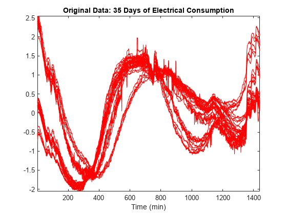
Load and Plot Multisignal
Load and plot a multisignal representing 35 days of an electrical load consumption. The data is centered and standardized. Observe that the signals are locally irregular and noisy but nevertheless three different general shapes can be distinguished.
load elec35_nor
X = signals;
[nbSIG,nbVAL] = size(X);
plot(X',"r")
axis tight
title("Original Data: 35 Days of Electrical Consumption")
xlabel("Time (min)")
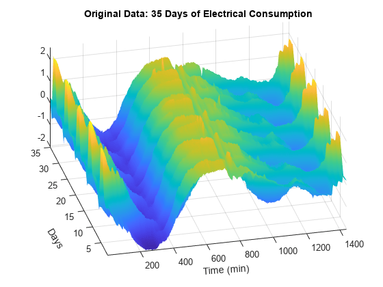
Surface Representation of Data
In order to highlight the periodicity of the multisignal, examine a 3-D representation of the data. The five weeks represented can be see more clearly.
surf(X)
shading interp
axis tight
title("Original Data: 35 Days of Electrical Consumption")
xlabel("Time (min)",Rotation=4)
ylabel("Days",Rotation=-60)
ax = gca;
ax.View = [-13.5 48];
Multisignal Row Decomposition
Use mdwtdec and perform a wavelet decomposition at level 7 using the sym4 wavelet.
dirDec = "r";         % Direction of decomposition
level  = 7;           % Level of decomposition
wname  = "sym4";      % Near symmetric wavelet
decROW = mdwtdec(dirDec,X,level,wname);
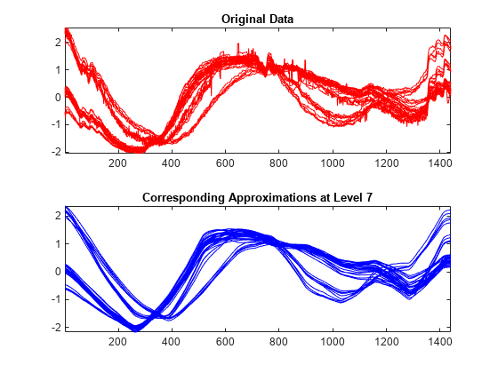
Signals and Approximations at Level 7
Reconstruct the approximations at level 7 for each row signal. Compare the approximations with the original signals. The approximations at level 7 capture the general shape, but some interesting features are lost. For example, the bumps at the beginning and at the end of the signals disappeared.
A7_ROW  = mdwtrec(decROW,"a",7);
tiledlayout(2,1)
nexttile
plot(X(:,:)',"r")
title("Original Data")
axis tight
nexttile
plot(A7_ROW(:,:)',"b")
axis tight
title("Corresponding Approximations at Level 7")
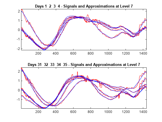
Superimposed Signals and Approximations
To compare more closely the original signals with their corresponding approximations at level 7, plot the original signals of the first four days superimposed with their corresponding approximations. Make an identical plot using the last five days of data. Note that the approximation of the original signal is visually accurate in terms of general shape.
tiledlayout(2,1)
idxDays = 1:4;
nexttile
plot(X(idxDays,:)',"r")
hold on
plot(A7_ROW(idxDays,:)',"b")
hold off
axis tight
title("Days "+int2str(idxDays))
nexttile
idxDays = 31:35;
plot(X(idxDays,:)',"r")
hold on
plot(A7_ROW(idxDays,:)',"b")
hold off
axis tight
title("Days "+int2str(idxDays))
Multisignal Denoising
To perform a more subtle simplification of the multisignal preserving these bumps which are clearly attributable to the electrical signal, denoise the multisignal.
The denoising procedure is performed in three steps:
Decomposition — Choose a wavelet and a level of decomposition N, and then obtain the wavelet decompositions of the signals at level N.
Thresholding — For each level from 1 to N and for each signal, a threshold is selected and thresholding is applied to the detail coefficients.
Reconstruction — Compute wavelet reconstructions using the original approximation coefficients of level N and the modified detail coefficients of levels from 1 to N.
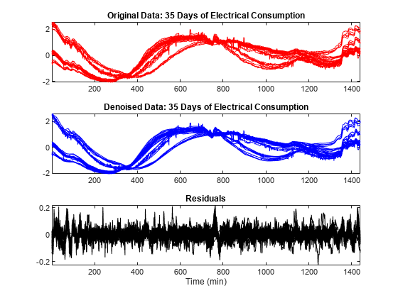
Use the mdwtdec and mswden functions to denoise the multisignal. Specify a level of decomposition N = 5 instead of N = 7 used previously. Note the bumps at the beginning and at the end of the signals are well recovered and, conversely, the residuals look like a noise except for some remaining bumps due to the signals. Furthermore, the magnitude of these remaining bumps is of a small order.
Tip: The output of mswden is used later in this example to demonstrate clustering. If you are only interested in denoising a multisignal, mswden is not recommended. Instead, use the wdenoise function.
dirDec = "r";         % Direction of decomposition
level  = 5;           % Level of decomposition
wname  = "sym4";      % Near symmetric wavelet
decROW = mdwtdec(dirDec,X,level,wname);

[XD,decDEN] = mswden("den",decROW,"sqtwolog","mln");
Residuals = X-XD;
figure
tiledlayout(3,1)
nexttile
plot(X',"r")
axis tight
title("Original Data: 35 Days of Electrical Consumption")
nexttile
plot(XD',"b")
axis tight
title("Denoised Data: 35 Days of Electrical Consumption")
nexttile
plot(Residuals',"k")
axis tight
title("Residuals")
xlabel("Time (min)")
Multisignal Compressing Row Signals
Like denoising, the compression procedure is performed using three steps (see above).
The difference with the denoising procedure is found in step 2. There are two compression approaches available:
The first approach consists of taking the wavelet expansions of the signals and keeping the largest absolute value coefficients. In this case, you can set a global threshold, a compression performance, or a relative square norm recovery performance. Thus, only a single signal-dependent parameter needs to be selected.
The second approach consists of applying visually determined level-dependent thresholds.
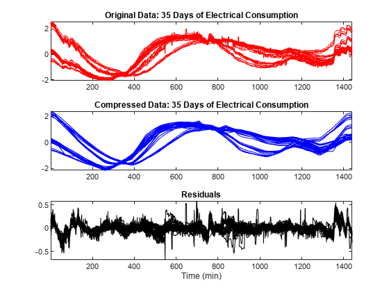
To simplify the data representation and to make more efficient the compression, use the mdwtdec and mswcmp functions. Compress each row of the multisignal by applying a global threshold leading to recover 99% of the energy. Specify a decomposition at level 7. The general shape is preserved while the local irregularities are neglected. The residuals contain noise as well as components due to the small scales essentially.
dirDec = "r";         % Direction of decomposition
level  = 7;           % Level of decomposition
wname  = "sym4";      % Near symmetric wavelet
decROW = mdwtdec(dirDec,X,level,wname);

[XC,decCMP,THRESH] = mswcmp("cmp",decROW,"L2_perf",99);
tiledlayout(3,1)
nexttile
plot(X',"r")
axis tight
title("Original Data: 35 Days of Electrical Consumption")
nexttile
plot(XC',"b")
axis tight
title("Compressed Data: 35 Days of Electrical Consumption")
nexttile
plot((X-XC)',"k")
axis tight
title("Residuals")
xlabel("Time (min)")
Compression Performance
Compute the corresponding densities of nonzero elements. For each signal, the percentage of required coefficients to recover 99% of the energy lies between 1.25% and 1.75%. This illustrates the capacity of wavelets to concentrate signal energy in few coefficients.
cfs = cat(2,[decCMP.cd{:},decCMP.ca]);
cfs = sparse(cfs);
perf = zeros(1,nbSIG);
for k = 1:nbSIG
    perf(k) = 100*nnz(cfs(k,:))/nbVAL;
end
figure
plot(perf,"r-*")
title("Percentages of Nonzero Coefficients for the 35 Days")
xlabel("Signal Indices")
ylabel("% of Nonzero Coefficients")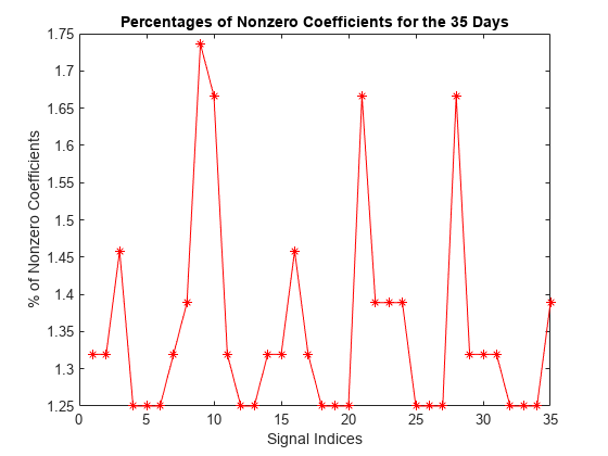
Clustering Row Signals
Clustering offers a convenient procedure to summarize a large set of signals using sparse wavelet representations. You can implement hierarchical clustering using the mdwtcluster function. You must have Statistics and Machine Learning Toolbox™ to use mdwtcluster.
Compare three different clusterings of the 35-day data. The first one is based on the original multisignal, the second one on the approximation coefficients at level 7, and the last one is based on the denoised multisignal.
Set to the number of clusters to 3. Compute the structures P1 and P2 which contain respectively the two first partitions and the third one.
P1 = mdwtcluster(decROW,"lst2clu",{'s','ca7'},"maxclust",3);
P2 = mdwtcluster(decDEN,"lst2clu",{'s'},"maxclust",3);
Clusters = [P1.IdxCLU P2.IdxCLU];
Confirm the equality of the three partitions.
EqualPART = isequal(max(diff(Clusters,[],2)),[0 0])
EqualPART = logical
   1
Plot and examine the clusters.
figure
stem(Clusters,"filled","b:")
title("The Three Clusters of the Original 35 days")
xlabel("Signal Indices")
ylabel("Index of Cluster")
ax = gca;
xlim([1 35])
ylim([0.5 3.1])
ax.YTick = 1:3;
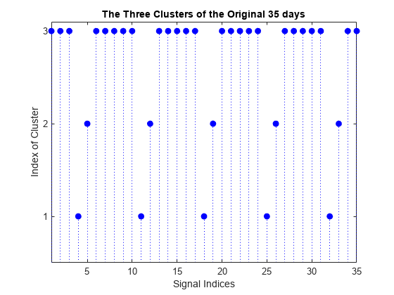
The first cluster (labelled 3) contains 25 mid-week days and the two others (labelled 2 and 1) contain five Saturdays and five Sundays respectively. This illustrates again the periodicity of the underlying time series and the three different general shapes seen in the two first plots displayed at the beginning of this example.
Display the original signals and the corresponding approximation coefficients used to obtain two of the three partitions.
CA7 = mdwtrec(decROW,"ca");
IdxInCluster = cell(1,3);
for k = 1:3
    IdxInCluster{k} = find(P2.IdxCLU==k);
end
%figure("Units","normalized","Position",[0.2 0.2 0.6 0.6])
figure
tiledlayout(3,2)
for k = 1:3
    idxK = IdxInCluster{k};
    nexttile
    plot(X(idxK,:)',"r")
    axis tight
    ax = gca;
    ax.XTick = [200 800 1400];
    if k==1
        title("Original Signals")
    end
    xlabel("Cluster: "+int2str(k)+" ("+int2str(length(idxK))+")")
    nexttile
    plot(CA7(idxK,:)',"b")
    axis tight
    if k==1
        title("Coefficients of Approximations at Level 7")
    end
    xlabel("Cluster: "+int2str(k)+" ("+int2str(length(idxK))+")")
end
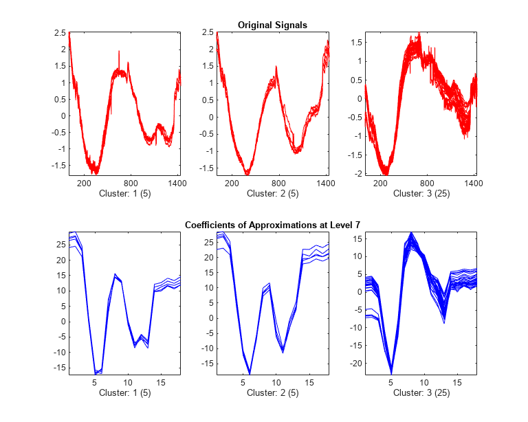
The same partitions are obtained from the original signals (1440 samples for each signal) and from the coefficients of approximations at level 7 (18 samples for each signal). This illustrates that using less than 2% of the coefficients is enough to get the same clustering partitions of the 35 days.
Summary
Denoising, compression and clustering using wavelets are very efficient tools. The capacity of wavelet representations to concentrate signal energy in few coefficients is the key of efficiency. In addition, clustering offers a convenient procedure to summarize a large set of signals using sparse wavelet representations. In this example, you used the mdwtdec and mswden functions to denoise the multisignal. You then used those results for clustering. If you are only interested in denoising, use instead the wdenoise function. The function provides a simple interface to a variety of denoising methods that can be applied to 1-D signals.