Main Content

wdenoise

Wavelet signal denoising

Description

example

XDEN = wdenoise(X) denoises the data in X using an empirical Bayesian method with a Cauchy prior. By default, the sym4 wavelet is used with a posterior median threshold rule. Denoising is down to the minimum of floor(log2N) and wmaxlev(N,"sym4") where N is the number of samples in the data. (For more information, see wmaxlev.) X is a real-valued vector, matrix, or timetable.

  • If X is a matrix, wdenoise denoises each column of X.

  • If X is a timetable, wdenoise must contain real-valued vectors in separate variables, or one real-valued matrix of data.

  • X is assumed to be uniformly sampled.

  • If X is a timetable and the timestamps are not linearly spaced, wdenoise issues a warning.

XDEN = wdenoise(X,LEVEL) denoises X down to LEVEL. LEVEL is a positive integer less than or equal to floor(log2N) where N is the number of samples in the data. If unspecified, LEVEL defaults to the minimum of floor(log2N) and wmaxlev(N,"sym4").

example

XDEN = wdenoise(___,Name,Value) specifies one or more options using name-value arguments in addition to any of the input arguments in previous syntaxes. For example, xden = wdenoise(x,3,Wavelet="db2") denoises x down to level 3 using the Daubechies db2 wavelet.

[XDEN,DENOISEDCFS] = wdenoise(___) returns the denoised wavelet and scaling coefficients in the cell array DENOISEDCFS. The elements of DENOISEDCFS are in order of decreasing resolution. The final element of DENOISEDCFS contains the approximation (scaling) coefficients.

[XDEN,DENOISEDCFS,ORIGCFS] = wdenoise(___) returns the original wavelet and scaling coefficients in the cell array ORIGCFS. The elements of ORIGCFS are in order of decreasing resolution. The final element of ORIGCFS contains the approximation (scaling) coefficients.

Examples

collapse all

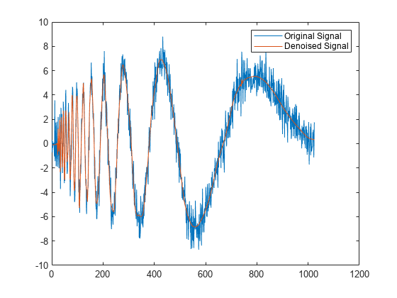
Obtain the denoised version of a noisy signal using default values.

load noisdopp
xden = wdenoise(noisdopp);

Plot the original and denoised signals.

plot([noisdopp' xden'])
legend("Original Signal","Denoised Signal")

Figure contains an axes object. The axes object contains 2 objects of type line. These objects represent Original Signal, Denoised Signal.

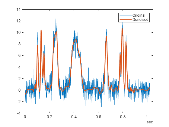
Denoise a timetable of noisy data down to level 5 using block thresholding.

Load a noisy dataset.

load wnoisydata

Denoise the data down to level 5 using block thresholding

xden = wdenoise(wnoisydata,5,DenoisingMethod="BlockJS");

Plot the original data and the denoised data.

h1 = plot(wnoisydata.t,[wnoisydata.noisydata(:,1) xden.noisydata(:,1)]);
h1(2).LineWidth = 2;
legend("Original","Denoised")

Figure contains an axes object. The axes object contains 2 objects of type line. These objects represent Original, Denoised.

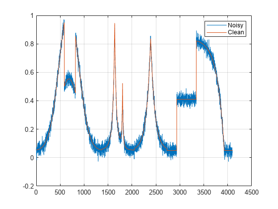
Denoise a signal in different ways and compare results.

Load a datafile that contains clean and noisy versions of a signal. Plot the signals.

load fdata
plot(fNoisy)
hold on
plot(fClean)
grid on
legend("Noisy","Clean")
hold off

Figure contains an axes object. The axes object contains 2 objects of type line. These objects represent Noisy, Clean.

Denoise the signal using the sym4 and db1 wavelets, with a nine-level wavelet decomposition. Plot the results.

cleansym = wdenoise(fNoisy,9,Wavelet="sym4");
cleandb = wdenoise(fNoisy,9,Wavelet="db1");
figure
subplot(2,1,1)
plot(cleansym)
title("Denoised - sym")
grid on
subplot(2,1,2)
plot(cleandb)
title("Denoised - db")
grid on

Figure contains 2 axes objects. Axes object 1 with title Denoised - sym contains an object of type line. Axes object 2 with title Denoised - db contains an object of type line.

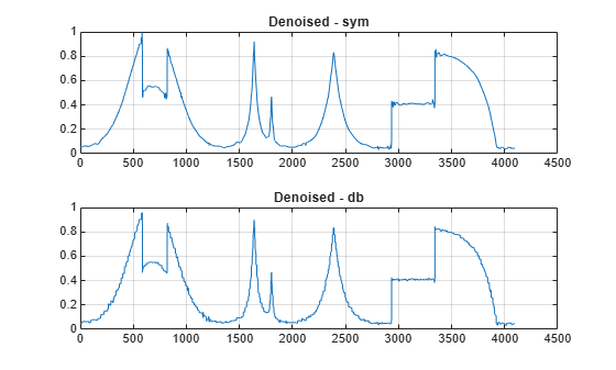
Compute the SNR of each denoised signal. Confirm that using the sym4 wavelet produces a better result.

snrsym = -20*log10(norm(abs(fClean-cleansym))/norm(fClean))
snrsym = 35.9623
snrdb = -20*log10(norm(abs(fClean-cleandb))/norm(fClean))
snrdb = 32.2672

Load in a file which contains noisy data of 100 time series. Every time series is a noisy version of fClean. Denoise the time series twice, estimating the noise variance differently in each case.

load fdataTS
cleanTSld = wdenoise(fdataTS,9,NoiseEstimate="LevelDependent");
cleanTSli = wdenoise(fdataTS,9,NoiseEstimate="LevelIndependent");

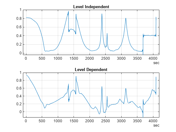
Compare one of the noisy time series with its two denoised versions.

figure
plot(fdataTS.Time,fdataTS.fTS15)
title("Original")
grid on

Figure contains an axes object. The axes object with title Original contains an object of type line.

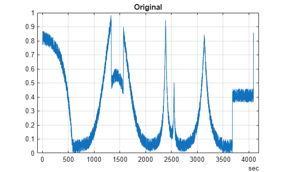
figure
subplot(2,1,1)
plot(cleanTSli.Time,cleanTSli.fTS15)
title("Level Independent")
grid on
subplot(2,1,2)
plot(cleanTSld.Time,cleanTSld.fTS15)
title("Level Dependent")
grid on

Figure contains 2 axes objects. Axes object 1 with title Level Independent contains an object of type line. Axes object 2 with title Level Dependent contains an object of type line.

Input Arguments

collapse all

Input data, specified as a matrix, vector, or timetable of real values. If X is a vector, it must have at least two samples. If X is a matrix or timetable, it must have at least two rows.

Data Types: double

Level of wavelet decomposition, specified as a positive integer. LEVEL is a positive integer less than or equal to floor(log2N) where N is the number of samples in the data.

  • If unspecified, LEVEL defaults to the minimum of floor(log2N) and wmaxlev(N,"sym4").

  • For James-Stein block thresholding, "BlockJS", there must be floor(log2N) coefficients at the coarsest resolution level, LEVEL.

Data Types: double

Name-Value Arguments

Specify optional pairs of arguments as Name1=Value1,...,NameN=ValueN, where Name is the argument name and Value is the corresponding value. Name-value arguments must appear after other arguments, but the order of the pairs does not matter.

Example: xden = wdenoise(x,4,Wavelet="db6") denoises x down to level 4 using the Daubechies db6 wavelet.

Before R2021a, use commas to separate each name and value, and enclose Name in quotes.

Example: "Wavelet","db6","DenoisingMethod","Bayes" denoises using the Daubechies db6 wavelet and the empirical Bayesian method.

Wavelet, specified as a character vector or string scalar. The wavelet must be orthogonal or biorthogonal. Orthogonal and biorthogonal wavelets are designated as type 1 and type 2 wavelets respectively in the wavelet manager, wavemngr.

  • Valid built-in orthogonal wavelet families are: Best-localized Daubechies ("bl"), Beylkin ("beyl"), Coiflets ("coif"), Daubechies ("db"), Fejér-Korovkin ("fk"), Haar ("haar"), Han linear-phase moments ("han"), Morris minimum-bandwidth ("mb"), Symlets ("sym"), and Vaidyanathan ("vaid").

  • Valid built-in biorthogonal wavelet families are: Biorthogonal Spline ("bior"), and Reverse Biorthogonal Spline ("rbio").

For a list of wavelets in each family, see wfilters. You can also use waveinfo with the wavelet family short name. For example, waveinfo("db"). Use wavemngr("type",wn) to determine if the wavelet wn is orthogonal (returns 1) or biorthogonal (returns 2). For example, wavemngr("type","db6") returns 1.

Denoising method used to determine the denoising thresholds for the data X.

  • Bayes — Empirical Bayes

    This method uses a threshold rule based on assuming measurements have independent prior distributions given by a mixture model. Because measurements are used to estimate the weight in the mixture model, the method tends to work better with more samples. By default, the posterior median rule is used to measure risk [8].

  • BlockJS — Block James-Stein

    This method is based on determining an `optimal block size and threshold. The resulting block thresholding estimator yields simultaneously optimal global and local adaptivity [3].

  • FDR — False Discovery Rate

    This method uses a threshold rule based on controlling the expected ratio of false positive detections to all positive detections. The FDR method works best with sparse data. Choosing a ratio, or Q-value, less than 1/2 yields an asymptotically minimax estimator [1].

  • Minimax — Minimax Estimation

    This method uses a fixed threshold chosen to yield minimax performance for mean square error against an ideal procedure. The minimax principle is used in statistics to design estimators. See thselect for more information.

  • SURE — Stein's Unbiased Risk Estimate

    This method uses a threshold selection rule based on Stein’s Unbiased Estimate of Risk (quadratic loss function). One gets an estimate of the risk for a particular threshold value (t). Minimizing the risks in (t) gives a selection of the threshold value.

  • UniversalThreshold - Universal Threshold 2ln(length(x)).

    This method uses a fixed-form threshold yielding minimax performance multiplied by a small factor proportional to log(length(X)).

Note

For "FDR", there is an optional argument for the Q-value, which is the proportion of false positives. Q is a real-valued scalar between 0 and 1/2, 0 < Q <= 1/2. To specify "FDR" with a Q-value, use a cell array where the second element is the Q-value. For example, "DenoisingMethod",{"FDR",0.01}. If unspecified, Q defaults to 0.05.

Threshold rule, specified as a character array, to use to shrink the wavelet coefficients. "ThresholdRule" is valid for all denoising methods, but the valid options and defaults depend on the denoising method. Rules possible for different denoising methods are specified as follows:

  • "BlockJS" — The only supported option is "James-Stein". You do not need to specify ThresholdRule for "BlockJS".

  • "SURE", "Minimax", "UniversalThreshold" — Valid options are "Soft" or "Hard". The default is "Soft".

  • "Bayes" — Valid options are "Median", "Mean", "Soft", or "Hard". The default is "Median".

  • "FDR" — The only supported option is "Hard". You do not need to define ThresholdRule for "FDR"

Method of estimating variance of noise in the data.

  • "LevelIndependent" — Estimate the variance of the noise based on the finest-scale (highest-resolution) wavelet coefficients.

  • "LevelDependent" — Estimate the variance of the noise based on the wavelet coefficients at each resolution level.

Specifying NoiseEstimate with the "BlockJS" denoising method has no effect. The block James-Stein estimator always uses a "LevelIndependent" noise estimate.

Output Arguments

collapse all

Denoised vector, matrix, or timetable version of X. For timetable input, XDEN has the same variable names and timestamps as the original timetable.

Data Types: double

Denoised wavelet and scaling coefficients of the denoised data XDEN, returned in a cell array. The elements of DENOISEDCFS are in order of decreasing resolution. The final element of DENOISEDCFS contains the approximation (scaling) coefficients.

Data Types: double

Original wavelet and scaling coefficients of the data X, returned in a cell array. The elements of ORIGCFS are in order of decreasing resolution. The final element of ORIGCFS contains the approximation (scaling) coefficients.

Data Types: double

Algorithms

The most general model for the noisy signal has the following form:

s(n)=f(n)+σe(n),

where time n is equally spaced. In the simplest model, suppose that e(n) is a Gaussian white noise N(0,1), and the noise level σ is equal to 1. The denoising objective is to suppress the noise part of the signal s and to recover f.

The denoising procedure has three steps:

  1. Decomposition — Choose a wavelet, and choose a level N. Compute the wavelet decomposition of the signal s at level N.

  2. Detail coefficients thresholding — For each level from 1 to N, select a threshold and apply soft thresholding to the detail coefficients.

  3. Reconstruction — Compute wavelet reconstruction based on the original approximation coefficients of level N and the modified detail coefficients of levels from 1 to N.

More details about threshold selection rules are in Wavelet Denoising and Nonparametric Function Estimation and in the help of the thselect function.

References

[1] Abramovich, F., Y. Benjamini, D. L. Donoho, and I. M. Johnstone. “Adapting to Unknown Sparsity by Controlling the False Discovery Rate.” Annals of Statistics, Vol. 34, Number 2, pp. 584–653, 2006.

[2] Antoniadis, A., and G. Oppenheim, eds. Wavelets and Statistics. Lecture Notes in Statistics. New York: Springer Verlag, 1995.

[3] Cai, T. T. “On Block Thresholding in Wavelet Regression: Adaptivity, Block size, and Threshold Level.” Statistica Sinica, Vol. 12, pp. 1241–1273, 2002.

[4] Donoho, D. L. “Progress in Wavelet Analysis and WVD: A Ten Minute Tour.” Progress in Wavelet Analysis and Applications (Y. Meyer, and S. Roques, eds.). Gif-sur-Yvette: Editions Frontières, 1993.

[5] Donoho, D. L., I. M. Johnstone. “Ideal Spatial Adaptation by Wavelet Shrinkage.” Biometrika, Vol. 81, pp. 425–455, 1994.

[6] Donoho, D. L. “De-noising by Soft-Thresholding.” IEEE Transactions on Information Theory, Vol. 42, Number 3, pp. 613–627, 1995.

[7] Donoho, D. L., I. M. Johnstone, G. Kerkyacharian, and D. Picard. “Wavelet Shrinkage: Asymptopia?” Journal of the Royal Statistical Society, series B, Vol. 57, No. 2, pp. 301–369, 1995.

[8] Johnstone, I. M., and B. W. Silverman. “Needles and Straw in Haystacks: Empirical Bayes Estimates of Possibly Sparse Sequences.” Annals of Statistics, Vol. 32, Number 4, pp. 1594–1649, 2004.

Extended Capabilities

Version History

Introduced in R2017b