Denoising Signals and Images

Soft or Hard Thresholding?

Thresholding can be done using the function wthresh which returns soft or hard thresholding of the input signal. Hard thresholding is the simplest method but soft thresholding has nice mathematical properties. Let thr denote the threshold.

thr = 0.4;

Hard thresholding can be described as the usual process of setting to zero the elements whose absolute values are lower than the threshold. The hard threshold signal is x if x > thr, and is 0 if x $\le$ thr.

y = linspace(-1,1,100); 
ythard = wthresh(y,'h',thr);

Soft thresholding is an extension of hard thresholding, first setting to zero the elements whose absolute values are lower than the threshold, and then shrinking the nonzero coefficients towards 0. The soft threshold signal is sign(x)(x-thr) if x > thr and is 0 if x $\le$ thr.

ytsoft = wthresh(y,'s',thr);
subplot(1,3,1)
plot(y)
title('Original')
subplot(1,3,2)
plot(ythard)
title('Hard Thresholding')
subplot(1,3,3)
plot(ytsoft)
title('Soft Thresholding')

As can be seen in the figure above, the hard procedure creates discontinuities at x = $$\pm$$ t, while the soft procedure does not.

Threshold Selection Rules

Recalling step 2 of the denoise procedure, the function thselect performs a threshold selection, and then each level is thresholded. This second step can be done using wthcoeff, directly handling the wavelet decomposition structure of the original signal. Four threshold selection rules are implemented in the function thselect. Typically it is interesting to show them in action when the input signal is a Gaussian white noise.

rng default
y = randn(1,1000);

Rule 1: Selection using principle of Stein's Unbiased Risk Estimate (SURE)

thr = thselect(y,'rigrsure')

thr = 
2.0518

Rule 2: Fixed form threshold equal to sqrt(2*log(length(y)))

thr = thselect(y,'sqtwolog')

thr = 
3.7169

Rule 3: Selection using a mixture of the first two options

thr = thselect(y,'heursure')

thr = 
3.7169

Rule 4: Selection using minimax principle

thr = thselect(y,'minimaxi')

thr = 
2.2163

Minimax and SURE threshold selection rules are more conservative and would be more convenient when small details of the signal lie near the noise range. The two other rules remove the noise more efficiently.

Let us use the "blocks" test data credited to Donoho and Johnstone as the first example. Generate original signal xref and a noisy version x adding a standard Gaussian white noise.

sqrt_snr = 4;      % Set signal to noise ratio
init = 2055615866; % Set rand seed
[xref,x] = wnoise(1,11,sqrt_snr,init);

First denoise the signal using wdenoise with default settings. Compare the result with the original and noisy signals.

xd = wdenoise(x);
subplot(3,1,1)
plot(xref)
axis tight
title('Original Signal')
subplot(3,1,2)
plot(x)
axis tight
title('Noisy Signal')
subplot(3,1,3)
plot(xd)
axis tight
title('Denoised Signal - Signal to Noise Ratio = 4')

Denoise the noisy signal a second time, this time using soft heuristic SURE thresholding on detail coefficients obtained from the decomposition of x, at level 3 by sym8 wavelet. Compare with the previous denoised signal.

xd2 = wdenoise(x,3,'Wavelet','sym8',...
    'DenoisingMethod','SURE',...
    'ThresholdRule','Soft');
figure
subplot(3,1,1)
plot(xref)
axis tight
title('Original Signal')
subplot(3,1,2)
plot(xd)
axis tight
title('First Denoised Signal: Default Settings')
subplot(3,1,3)
plot(xd2)
axis tight
title('Second Denoised Signal')

Since only a small number of large coefficients characterize the original signal, both denoised signals compare well with the original signal. You can use the Wavelet Signal Denoiser to explore the effects other denoising parameters have on the noisy signal.

Dealing with Non-White Noise

When you suspect a non-white noise, thresholds must be rescaled by a level-dependent estimation of the level noise. As a second example, let us try the method on the highly perturbed part of an electrical signal. Let us use db3 wavelet and decompose at level 3. To deal with the composite noise nature, let us try a level-dependent noise size estimation.

load leleccum
indx = 2000:3450; 
x = leleccum(indx); % Load electrical signal and select part of it.

Denoise the signal using soft fixed form thresholding and level-dependent noise size estimation.

xd = wdenoise(x,3,'Wavelet','db3',...
    'DenoisingMethod','UniversalThreshold',...
    'ThresholdRule','Soft',...
    'NoiseEstimate','LevelDependent');
Nx = length(x);
figure
subplot(2,1,1)
plot(indx,x)
axis tight
title('Original Signal')
subplot(2,1,2)
plot(indx,xd)
axis tight
title('Denoised Signal')

The result is quite good in spite of the time heterogeneity of the nature of the noise after and before the beginning of the sensor failure around time 2410.

Image Denoising

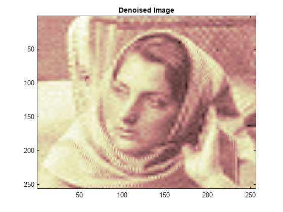
The denoising method described for the one-dimensional case applies also to images and applies well to geometrical images. The two-dimensional denoising procedure has the same three steps and uses two-dimensional wavelet tools instead of one-dimensional ones. For the threshold selection, prod(size(y)) is used instead of length(y) if the fixed form threshold is used.

Generate a noisy image.

load  woman 
init = 2055615866;
rng(init); 
x = X + 15*randn(size(X));

In this case fixed form threshold is used with estimation of level noise, thresholding mode is soft and the approximation coefficients are kept.

[thr,sorh,keepapp] = ddencmp('den','wv',x);
thr

thr = 
107.9838

Denoise image using global thresholding option.

xd = wdencmp('gbl',x,'sym4',2,thr,sorh,keepapp);
figure('Color','white')
colormap(pink(255))
sm = size(map,1);
image(wcodemat(X,sm))
title('Original Image')

figure('Color','white')
colormap(pink(255))
image(wcodemat(x,sm))
title('Noisy Image')

image(wcodemat(xd,sm))
title('Denoised Image')

Summary

Denoising methods based on wavelet decomposition is one of the most significant applications of wavelets. See wdenoise and Wavelet Signal Denoiser for more information.