Image Pyramid
This example shows how to generate multi-level image pyramid pixel streams from an input stream. This model derives multiple pixel streams by downsampling the original image in both the horizontal and vertical directions using Gaussian filtering. This type of filter avoids aliasing artifacts. The implementation uses an architecture suitable for FPGAs.
Image pyramid is used in many image processing applications such as image compression, object detection, and object recognition that use techniques such as convolutional neural network (CNN) or aggregate channel features (ACF). Image pyramid is also similar to scale-space representation.
The example model takes a 240p video input and produces three output streams: 160x120, 80x60, and 40x30.
modelname = 'ImagePyramidHDL';
open_system(modelname);
set_param(modelname,'SampleTimeColors','on');
set_param(modelname,'SimulationCommand','Update');
set_param(modelname,'Open','on');
set(allchild(0),'Visible','off');
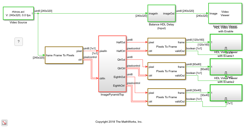
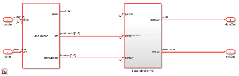
Each level of the pyramid contains a Line Buffer block and a downsampling filter.
open_system([modelname '/ImagePyramidTop/GaussianPyramidDownsample'],'force');
Filter Coefficients
The approximate Gaussian filter coefficients in [1] have been used in a number of image pyramid implementations. These coefficients are given by:
format long
Hh = [1 4 6 4 1]./16;
Hv = Hh';
Hg = Hv*Hh
Hg =

  Columns 1 through 3

   0.003906250000000   0.015625000000000   0.023437500000000
   0.015625000000000   0.062500000000000   0.093750000000000
   0.023437500000000   0.093750000000000   0.140625000000000
   0.015625000000000   0.062500000000000   0.093750000000000
   0.003906250000000   0.015625000000000   0.023437500000000

  Columns 4 through 5

   0.015625000000000   0.003906250000000
   0.062500000000000   0.015625000000000
   0.093750000000000   0.023437500000000
   0.062500000000000   0.015625000000000
   0.015625000000000   0.003906250000000
The results are similar to but not exactly the same as the Gaussian kernel with a 1.0817797 standard-deviation. So, Hg is an approximate Gaussian kernel.
Hf = fspecial('gaussian',5,1.0817797)
Hf =

  Columns 1 through 3

   0.004609023214619   0.016606534868404   0.025458671096979
   0.016606534868404   0.059834153028525   0.091728830511040
   0.025458671096979   0.091728830511040   0.140625009648116
   0.016606534868404   0.059834153028525   0.091728830511040
   0.004609023214619   0.016606534868404   0.025458671096979

  Columns 4 through 5

   0.016606534868404   0.004609023214619
   0.059834153028525   0.016606534868404
   0.091728830511040   0.025458671096979
   0.059834153028525   0.016606534868404
   0.016606534868404   0.004609023214619
The filter, Hg, is obviously separable because it is constructed from horizontal and vertical vectors. Therefore, a separable filter implementation is a good choice. Many of the coefficient values are powers of two or a combination of only two powers of two. These values mean that the filter implementation can replace multiplication with shift and add techniques such as canonical signed digit (CSD). Each vector in the separable representation is also symmetric, so the filter implementation uses a symmetry pre-adder to further reduce the number of operations.
Downsampling
After low-pass filtering with the approximate Gaussian filter above, the model then downsamples the pixel stream by two in both the horizontal and vertical directions. To downsample, the model alternates the valid signal to be high only for every other pixel. The model also recreates the other pixelcontrol bus signals.
The model includes horizontal and vertical counters that compare the number of output pixels and lines with the mask parameters for active pixels and lines. The model uses these counts to recreate the end of line (hEnd) and end of frame (vEnd) signals.
After downsampling once, the pixelcontrol bus valid signal alternates high and then low every other pixel. After the second downsample, it alternates with a pattern of one valid pixel followed by three non-valid pixels. In some applications, you may want to collect all the valid pixels into a continuously valid period of time. The Pixel Stream FIFO block, used between downsample stages, produces continuous valid pixels for each line.
Each GaussianPyramidDownsample subsystem accepts parameters for the input frame size and decimation factor. These numbers must be integers and the decimation factor a power of 2. If the input number of pixels per line is odd rather than even, then round down to the next integer. For example, if the input size is 25 pixels per line, the specified input size must be 24 pixels per line.
Going Further
The Gaussian filter kernel used in a traditional image pyramid is not the only low-pass filter that could be used. Using an edge-preserving low-pass filter, such as a bilateral filter with different kernel sizes, would preserve more detail in the pyramid.
It is sometimes helpful to compute the difference between two levels of an image pyramid. This algorithm is called a Laplacian pyramid. The smaller level is upsampled to the same size as the larger level and filtered. The filter is usually a scaled version of the same approximate Gaussian filter used in this model. The difference between layers represents the information lost in the downsampling process. A Laplacian pyramid can be used for applications including coring for noise removal, compositing images taken at different times or with different focal lengths, and many others.
A potential limitation of this model is that there is fairly high latency between the output streams. This latency occurs because the second and third levels depend on the output from the previous level. This latency could be avoided by creating parallel filters that operate on more lines. This example implements a 5-by-5 filter that stores 5 lines at each level. A lower-latency parallel implementation requires 13 lines of storage for a two-level filter or 103 lines for a three-level filter. This is not generally a cost-effective trade-off.
On FPGAs, line buffer memories are typically implemented using block RAMs. Smaller memories can be implemented in the FPGA fabric and are known as distributed RAMs. Your synthesis tool chooses block or distributed RAM depending on the resources of your device. As the line size becomes smaller due to downsampling, distributed RAMs can be more efficient. In this example, the Line Buffer blocks in each level reserve space based on their Active pixels per line rounded up to next power of 2. For the example's 240p input the line buffer sizes are 512, 256, and 128.
References
[1] Burt, P., and E. Adelson. "The Laplacian Pyramid as a Compact Image Code."IEEE Transactions on Communications 31, no. 4 (April 1983): 532-40.